Nowadays, video surveillance systems are used for traffic control. Many organizations, buildings, and houses have security cameras, but the resolution and quality of these cameras are insufficient because the cameras record and store all captured video on hard drives, which are expensive. In order to store recorded video at high quality, there is a need to have a huge number of volumes, which are not affordable by many. Accordingly, these systems create difficulties in video analysis by producing low-quality outputs. Captured videos and photos frequently appear blurred, distorted, or fuzzy. Digital image processing techniques are used to overcome this problem.
2. Digital Image Representation
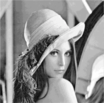
It is important to discuss image representation in computers in order to understand image-processing algorithms, which are used in the project. First, let us talk about images in
This is a way of wrapping colors of an image into its brightness values. The representation of color images will be discussed later, but their constructions are accomplished in the same manner with little difference.
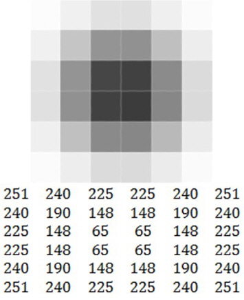
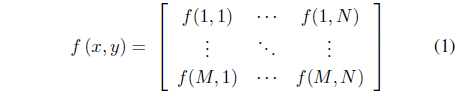
Grayscale images are constructed by a two-dimensional light intensity function
The matrix is the representation of the image of Figure 2 in the spatial domain. Each value of the matrix at (
There is also a
RGB: image contains three channels, and color at a pixel is represented by a set of three colors (red, green, and blue); CMYK: image has four channels, and the color of a pixel is a vector containing the colors cyan, magenta, yellow, and black; HSV (hue-saturation-value): stores color information in three channels, just like RGB, but one channel is for a brightness value and the other two store color information.
Images in this project are processed as RGB images.
A
As mentioned above, the digitized brightness value is called a gray level or grayscale. Each element in the array is called a pixel. One image may contain one to several dozen pixels.
The mathematical representation of a digital image looks like this [3]:
Usually, most image processing algorithms refer to gray images. There are various reasons:
All operations applied to gray images can be extended to color images by applying that method for each channel of an image; A lot of information can be extracted from a gray image, and colors might be not necessary; Handling one channel takes less CPU time; For many years, images were black and white. Therefore, most algorithms have been created for this type of image.
There are many other reasons for using gray scaled images in image processing, but the list above shows the most important ones.
Along with the digitization of images, image processing has been developed to solve problems. Many image processing tools, techniques, and algorithms have been created. Not many people completely understand what image processing is and why we need it. Why do we need image processing?
There are three major problems that paved the way for the development of image processing [3]:
Picture digitization and creating coding standards to make transmission and storing easier; Image restoration and making enhancements for further interpretations, for example, refining pictures of surfaces of other planets; Image segmentation and preparation for machine vision.
Nowadays, image processing concerns operations mainly on digital images. This is a branch of science called computer vision[3-5]. Computer vision is an important key for robotics and machine learning.
In image processing, there might be a need for image enhancements to overcome physical limits such as camera resolution and degradation. Image enhancement is the process of improving an image by making the image look better [3]. Actually, we do not know how the image should finally look like, but it is possible to say whether the image is improved by considering whether more detail can be seen or unwanted noise has been removed. Therefore, an image is enhanced when we have removed additive noise, increased the contrast, and decreased blurring.
In addition, when we scale up an image, it loses its quality and some details are unrecognizable. In order to avoid this, there is a need for super-resolution techniques, which allow restoring of the image after its transformations.
This project includes two types of image enhancements: restoring a blurred image and super-resolution.
2.2.1 Blurred image restoration
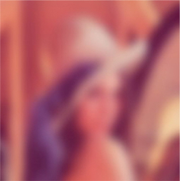
Restoring distorted images is one of the important problems in image processing. A specific case is blurring owing to improper focus, which is familiar to everyone. In addition to this type of degradation, there is also noise, incorrect exposition, and so on, but all of them can be restored using any image editing software.
The image below is an example of a blurred image (Figure 3).
It is believed by many that image blurring is an irreversible operation and that information is permanently lost and cannot be restored. Because each pixel is converted into a spot, everything is mixed, and with a large radius of blur we get uniform color through the entire image. However, this is inaccurate. All information is simply distributed according to some law, and can be uniquely recovered with some reservations. The only exception is the width of the image in the blur radius; full recovery is not possible for this characteristic.
Let us examine a more formal and scientific description of image degradation and restoration processes. Only gray scaled images will be reviewed, considering that color images can be handled in the same way for each color channel [1, 2, 4]. First we define the following notations:
f(x, y): Initial clear image h(x, y): Degradation function n(x, y): The additive noise term g(x, y): Degraded image
The degraded image is produced by the following formula:

As seen from the formula, image degradation is achieved by the convolution of the initial image with a degradation function.
The objective of restoration is to obtain an estimate
In the degradation process, each pixel turns into a spot, and into a section in the case of a simple blur. Alternatively, each pixel of the degraded image is obtained by pixels from some neighboring regions. All of these pixels construct the degraded image. The law of distribution for pixels is called the degradation function. The degradation function is also known as a point spread function (PSF) or kernel [6]. Usually the size of kernel function is less than the size of the initial image. In the example where we have degraded and restored a one-dimensional image, the size of the kernel was equal to two, i.e., each pixel was obtained from two.
Let us demonstrate using an example of a one-dimensional image:
The initial image is [
After applying a blur, each pixel sums with the neighboring left pixel: .
Accordingly, we get a blurred image:[
Next, we try to restore the image. In order to do this, we have to subtract from second pixel the value of the first pixel, from the third one the result of the previous subtraction, and so on.
The restored image: [
Here we have added an unknown constant value
Noise in digital images occurs because of image digitization or transmission. Digital camera sensors can be affected by environmental conditions, or the problem might be in the performance of the sensor itself. For instance, while taking a picture with a digital camera, the temperature and light levels can affect the resulting image. Transmission of an image through wireless networks can also corrupt the image by atmospheric disturbance. In most cases, the noise that appears is Gaussian (also called
“Super-resolution” (SR) is a term used to describe a part of image processing methods that is designed to enhance the image and fetch a high-resolution image from one or multiple low-resolution (LR) images. Image processing programmers or researchers frequently ask what super-resolution is. Most of the time it is explained by using an example from movies about CSI or the FBI where an agent looks at a LR image and pushes the magic “enhance” button, and then the LR image becomes clear and readable. This method from TV shows is an example of SR.
The images may appear at insufficient resolutions for several reasons. They may be taken from a great distance, for example, an area photo taken by a satellite. The images may have been recorded without knowing what objects are important. These kinds of problems often appear in security camera recordings, which are positioned to record a crowd of people or a large area. Sometimes it appears that the images are taken with LR imaging sensors of cell phone cameras.
There are two approaches to achieve SR images: single-image SR and multiple-image super-resolution. As their names denote, the single-image SR method needs only one LR image to get the SR image, and multiple-image SR needs several LR images of the same scene with slight shift to achieve the desired result. In this project, multiple-image SR is used.
In order to understand SR techniques, it is important to know about the formation of LR images. Typically, a set of LR images is recorded sequentially by a single camera. Usually there is a little motion between any pair of frames from the observing LR images, and they are blurred while passing through the system of a camera. Finally, the set of initial images is sampled at a relatively low spatial frequency. Additive noise makes the images even worse.
In this model of LR image formation, the LR image is taken from a high-resolution image by applying three linear operators and adding noise. For example, let us take a high-resolution image of a scene as

In the formula for the LR image,
The process of obtaining a high-resolution image from the LR image or a set of LR images requires a basic technique from image processing for image transformations. The variable
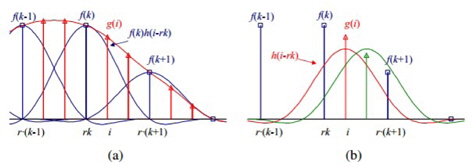
The most useful transformation in this project is
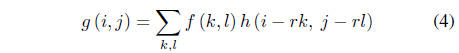
This formula (4) is related to the discrete convolution formula, but indexes
These two forms are equivalent, and the second form is also called a
There are different types of kernels, which are used depending on the application and computational time.
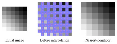
Figure 5 [7] shows how the nearest-neighbor method works. This type of interpolation copies the nearest pixel values by just enlarging the pixels.
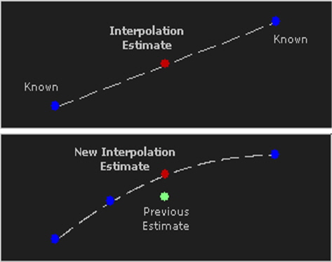
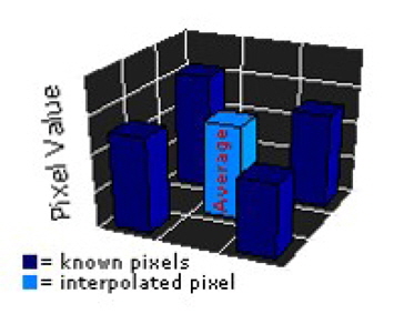
The estimation value is more precise when more values are known. In the image on the left there are two known points, and the estimation point is located in the center. It can be clearly seen in the right picture how estimation becomes more accurate when a new known point is added. Bilinear interpolation uses the same principle, but the interpolating process occurs in three dimensions. This can be seen in Figure 7 [7].
The types of interpolations were listed from less to more complex in consuming processing time and implementation. The results of interpolations become more applicable to many areas.
3.2 Multiple-Image Super-resolution
The main difference between multiple-image SR and the described interpolation methods in the previous section is that the final result of the former is constructed by observing LR images. For the latter new pixel values are just averaged from neighboring areas. In order to obtain a high-resolution image from multiple LR images, it is important to know more information about observed LR images. For example, if we know the motion estimates of a set of LR images, then we know where to plot every pixel of each LR observation image on the high-resolution [8].
Image processing and pattern recognition techniques are helpful in analyzing images, pattern classification, image restoration, and recognition. Since a great number of techniques have been proposed, the choice of appropriate technique for a specific task is important. This paper can be used as the first step in working with image processing. Thus, for a specific task, we may need to develop a new technique. This will be made possible by the collaboration of researchers in image processing and pattern recognition. In future, we will improve image processing and restoration algorithms using image digitization and mathematical algorithms.


![Example of interpolation using the nearest-neighbor method [7].](http://oak.go.kr/repository/journal/17132/E1FLA5_2015_v15n3_172_f005.jpg)
![Linear interpolation scheme [7].](http://oak.go.kr/repository/journal/17132/E1FLA5_2015_v15n3_172_f006.jpg)
![Bilinear interpolation [7].](http://oak.go.kr/repository/journal/17132/E1FLA5_2015_v15n3_172_f007.jpg)
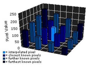
![Bicubic interpolation [7].](http://oak.go.kr/repository/journal/17132/E1FLA5_2015_v15n3_172_f008.jpg)