The navigation problem of mobile robots is one of the most popular issues in robot field. Mobile robots have been used and performed some risky and repetitive tasks for human being, such as space research, factory automation and defense security, which economized the labor force to be engaged in other aspects. In these areas, how to detect the surrounding information and guide the movement of mobile robots has become a primary question. So in an environment with obstacles, a mobile robot should have a fundamental skill of finding a collision-free path from a starting location to a planned target location.
In the past few decades, plenty of researchers have applied their energy to solve the navigation problem of mobile robots. Such as, in [1], the researchers proposed a control rule to find out reasonable target linear and rotational velocities of the mobile robot using PID controllers. Moreover, in [2], the authors used only artificial vision to establish both the robots position and orientation relative to the target using non-linear controllers based on Lyapunov stability analysis. The soft computing methods also have been tried to solve this problem such as fuzzy logic, genetic algorithm (GA), neural network, etc. The artificial neural network (ANN) has the ability to learn the situations of the environment. Many researchers have applied the neural network [3, 4] successfully to develop the methods of the navigation problem of a mobile robot. In [5], GAs together with characteristics has the ability in solving such problems and they can approach for optimum results in environment with dynamic obstacles. The fuzzy logic controller (FLC) for the navigation and obstacle avoidance problem of mobile robots also has been studied by many researchers for years. One of the most important questions is to establish a high-efficiency rule set. The performance of FLC is influenced by its knowledge base (rule set) and the membership functions. Thus, it is indispensable to adjust the rules of fuzzy controller and the membership functions of input and output variables to get a better performance. In [6], a GA was applied to modify the input and output membership functions of the fuzzy controller. Researches in [7] combined the fuzzy logic with both GA and ANN for path planning problem of mobile robot in static environment, and three different algorithms were loaded with different effects. Many other researchers [8] have also applied the GA optimized FLC in this area. But most of them used the regular (circle shape) obstacles for simulation. In the environment with irregular obstacles, these methods might not work properly. Here, we studied the navigation problem of a wheel mobile robot in the unknown environment with both regular and irregular obstacles based on proximity sensors by FLC. Then a GA was applied to optimize both the membership functions and the rules set of the fuzzy controller. In the case of path deadlock problem, a wall following method was also proposed.
The rest of this paper is organized as follows: Section 2 presents the modeling of the robot and kinematic functions. Section 3 describes the FLC. In Section 4, we present an optimization method for FLC by GA. Section 5 presents a strategy of exploring the way forward and a wall following method. In Section 6, we verify the effectiveness of the proposed method by simulation. Finally, conclusions and discussions are included in Section 7.
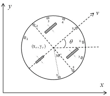
In order to obtain the required information of environment for navigation, different kinds of mobile robots with different sensors have been used for this purpose. In this work, we choose a classic wheeled robot as an example for simulation, which has two DC motors for left and right wheel and both wheel has an encoder on each one so that the robot can detect how far each motor has moved by itself. As shown in Figure 1, the robot has nine proximity sensors (ultrasonic sensors or infra-red sensors). Totally three groups of sensors have been installed at the front, left side and right side of the robot. Every group has three sensors, and every sensor has been setup for every 30 degrees. These sensors are used to detect the distance to the surrounding obstacles. We assume that the position of all the obstacles is unknown and the start and goal position are known for the robot.
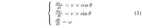
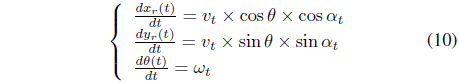
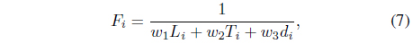
To simplify the simulation, we put two wheels together to consider as the unicycle. Thus, the kinematic functions can be described as the following equations:

where (
3. Design of Fuzzy Logic Controller
Fuzzy logic control is one of the most successful areas in the application of intelligent control. The fuzzy logic control theory has shown excellent performance when the processes are too complex for analysis by traditional mathematical description [9]. It includes three components which are fuzzification, fuzzy inference and defuzzification.
The fuzzification process can be used to transforms a non-fuzzy input value to a fuzzy value. As an example, in this work, there are two input variables:


where
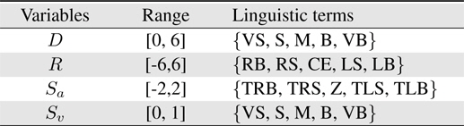
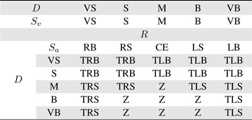
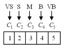
For fuzzifier, the input and output values which with the corresponding range, can be divided into five linguistic terms as shown in Table 1.
[Table 1.] Variable range and linguistic terms

Variable range and linguistic terms
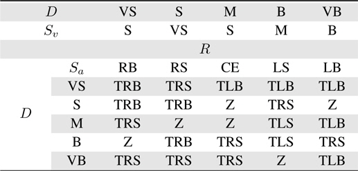
Here, the meaning of every linguistic values respectively are: very small (VS), small (S), middle (M), big (B), very big (VB), right big (RB), right small (RS), center equal (CE), left small (LS), left big (LB), turn right big (TRB), turn right small (TRS), zero (Z), turn left small (TLS) and turn left big (TLB).
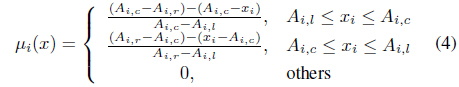
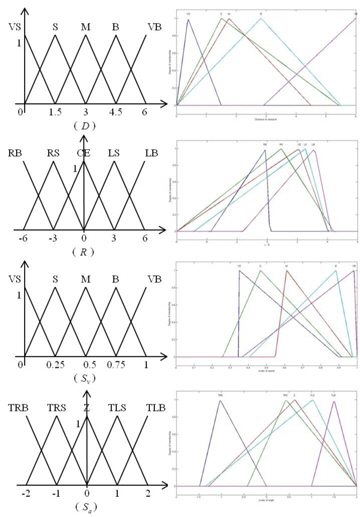
The transformation process of non-fuzzy input values to fuzzy values is achieved by using the membership functions which provide fuzzy terms with a definite meaning [10]. In this work, we used the triangular membership functions. For the

The process of fuzzy inference usually uses a set of rules to appoint the desired control behavior. A rule is a condition description take the form of IF...AND...THEN... rules. The rules set used here are as shown in Table 2. Specially, when the distance difference
[Table 2.] Rules set of fuzzy logic controller

Rules set of fuzzy logic controller
The rules set and membership functions discussed in Section 3 were created all by human experience, which will influence the performance of a FLC. Thus, it is indispensable to adjust them to get a better performance. A GA is employed here to do this work. A GA is a search strategy based on models of evolution in nature. A GA requires several steps including generating an initial population made up of chromosomes (candidate solutions to the optimization problem), calculating a fitness value for each chromosome, finding the best set of chromosomes that will be used to form the next generation, perform a reproduction selection on the other chromosomes, performing some diversity for the next generation using crossover and mutation, and continuing with the next generation until some stopping criterion is met. Therefore we can achieve the proposed optimization procedure in accordance with the following order.
a) Chromosomes and initialization
A chromosome corresponds to a possible solution of the optimization problem and every chromosome is composed of several encoded genes. In order to encode a FLC, we integrated the proposed encoding procedure with both the membership functions and rules set. We use
GAs are efficient techniques for searching for global optimum solutions but may have premature convergence problems [11]. In our case, the number of original individuals of the first generation is initialized as 30. In order to improve the convergence rate of GA and avoid the premature convergence, we added three same individuals which generated by the input and out values and rules set discussed in the previous section. The rest 27 individuals are produced randomly with real number coding format.
b) Fitness function
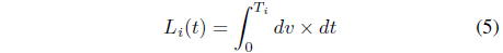
In our case, a feasible fitness function should include two elements, that is, efficiency and security. Thus, for the
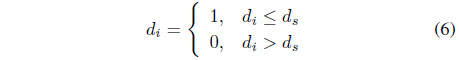
A penalty function is required to insure that the robot will not collision any obstacles. Denote that
Then the fitness function can be written as:
where
c) GA operators
In the proposed algorithm, we used three traditional GA operators: selection, crossover and mutation. Here the ‘stochastic universal sampling’ (SUS) is used as the selection operator. Moreover, the ‘double-point crossover operator’ and ‘realvalued mutation operator’ were used for crossover and mutation procedure in this work.
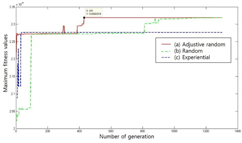
By following the above steps, now we can implement the optimization procedure. Several essential parameters are defined as: crossover rate is 0.9, mutation rate is 0.01 and maximum generation is 1300. Therefore, through the evolution, we can get the curves of the changing of the maximum fitness values in every generation as shown in Figure 4.
In Figure 4, we compared three different initialization methods: curve (a) is the method which used 3 experiential individuals generated by the FLC controller discussed in Section 3 and 27 random generated individuals. The result with completely random generated 30 individuals is shown as curve (b). Moreover, curve (c) is generated by completely experiential 30 individuals. From these curves we can see that curve (a) shows the maximum fitness value at the 431th generation, which is the fastest. Because of the lacking of population diversity, curve (c) prematurely fall into local extremum. Hence, these 3 empirically generated individuals can improve the convergence speed and insure the diversity of population at the same time.
The optimized membership functions compared with the original ones are shown in Figure 5. Table 3 describes the evolved rules set from Table 2.
[Table 3.] Evolved fuzzy rules set
Evolved fuzzy rules set
5. Obstacle Avoidance and Wall-Following Method
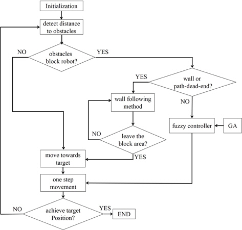
Our purpose is to guide the mobile robot with a collision-free path to move in multi-obstacle environment and reach the target position successfully. Firstly, the robot will rotate towards the target and move ahead with the maximum speed. Once the sensors detect any obstacle block the way, a FLC is to be activated. Figure 6 described the flowchart of the process of obstacle avoidance using the proposed algorithm. Specially, if there is a wall on the way of robot or a u-valley deadlock condition, the wall following method which will be discussed here will be used to find a way to escapes out.
Refer to the coordinates system shown in Figure 1, at time


where

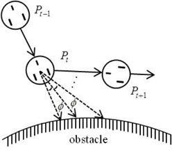
In order to ensure safety, before the robot moves ahead, firstly the robot will check whether the distance between the robot body and obstacles is far enough than the safety distance. As shown in Figure 7, the robot has moved from the position

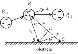
In the special case with big obstacles (or a wall) or a deadlock condition (e.g., u-valley obstacle), the robot might be guide further and further from the goal position or moves back and forth inside the u-valley obstacle. Thus, if the robot can move along the edge of the obstacle until leave the block area, it will be able to escape the problem. As shown in Figure 8, a wall following method named angle compensation method was developed here.
As shown in Figure 8, we assume that the current position of the robot is
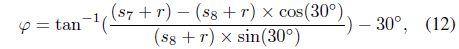
where
In order to verify the effectiveness of the algorithm we have discussed, a series of simulations have been implemented with Matlab. The multi-obstacle environment was set as 100 × 100 unit-length, and the start and goal position are (0, 0) and (100, 100) respectively. The accelerated speed wont be considered, and the radius and the maximum speed of the robot are set as 1.5 unit-length and 4 unit-length per second. We will record the position of the robot by every 0.5 second. Both the regular (circle shape) and irregular (geometrical shape) obstacles have been simulated in this work.
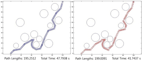
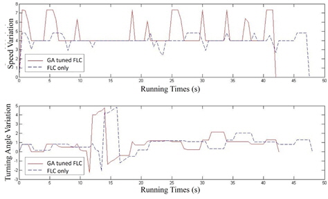
The results in the environment with regular obstacles are shown in Figures 9 and 10. In this case, we only consider the periphery of each obstacle, which can be described by a circle shape. As shown in Figure 9, the obstacles (circle) are much bigger than the robots radius. Thus, when the robot is too close to the obstacles the proposed wall following method will be activated. Compare the path generated by evolved and un-evolved FLC, we can find that the evolved FLC demonstrated almost useless to shorten the path length. However, the running time has been observably decreased from 47.7938 to 41.7437 seconds. Compared with the results of performance gain (7.63% in running time) in [6] and that (1.72% in path length) in [8], the method proposed in this work can get the 12.66% of performance improvement, which should be more effective. Similarly, in Figure 10, the amplitude variation of turning angle over the whole path was not obvious before and after evolution. Nevertheless, the velocity was increased.
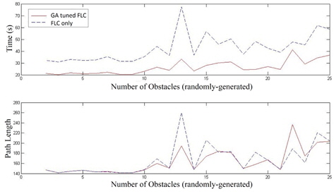
In order to verify our analysis, a series of simulations have been achieved with different numbers (form 2 to 25) of circle shape obstacles (see Figure 11). From this figure we can see that no matter how many obstacles there are the running time has obviously reduced by the optimized FLC. These simulations, out the other side, proved that the proposed wall following method demonstrated excellent performance in obstacle avoidance and smoothness of the path.
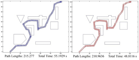
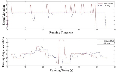
The simulation results with irregular obstacles are shown in Figures 12 and 13. In Figure 12, the simulation with several irregular obstacles composed by different kinds of geometrical shapes was performed. Here, the running time of the robot is decreased from 55.1929 to 48.8116 seconds.
This paper studied a navigation problem with path planning for the mobile robot in unknown environment using FLC and GA. The information of environment and the distance between the robot body and obstacles were detected all by the robots own sensors. A GA was used to optimize the membership functions and rules set of FLC. The simulation results showed that the FLC and proposed wall following method have excellent performance in path planning and obstacle avoidance process. Compare the paths generated by the optimized and unoptimized fuzzy controller the running time of the navigation procedure was observably decreased.
In this work, all the obstacles were fixed with certain position. Future research will focus on extending the algorithm to an environment with dynamic obstacles. In addition, more experiments can be done by applying the proposed method to a real robot.