With the rapid development of wireless communication, microelectronics, and embedded computing technologies, sensor networks are widely used in certain fields, such as the military, environment, and medicine. Therefore, nowadays, these networks have become a popular topic of research. In a wireless sensor network, sensors always communicate with the server and other sensors (e.g., for sending data or accepting data). However, in the process of communication, we can expect the transmitted sensor data to get lost or corrupted for many reasons, such as bad weather conditions, the sensor node’s communication ability, wireless signal strength, power outage at the sensor node, or a relatively high bit error rate of the wireless radio transmissions as compared with wired communications. In general, we can re-query data or discard data, but re-querying data is a naive alternative as it may induce a long wait or quicken the power exhaustion of the node, and most importantly, it does not guarantee having the original reading available. Discarding data is also a bad choice as it may lead to the loss of some interesting data. Therefore, it is essential to develop a technique for estimating missing data.
Data mining can produce knowledge from the existing data, and this knowledge can be used for estimating the missing sensor data. However, the existing missing sensor data estimation approaches do not achieve good results (as discussed in the following section). Therefore, in this paper, we propose a new estimation model based on a spatial-temporal correlation analysis (STCA). This model can discover intrinsic relationships among sensors and then incorporate the intrinsic relationships and the spatial-temporal relationship into data estimation. Finally, STCAM is tested with data from a traffic monitoring sensor application.
In fact, the topic of missing data estimation belongs to the field of statistics, and many researchers have conducted a considerable amount of research on this topic by using methods such as mean substitution, linear regression, Bayesian estimation, expectation maximization, k-nearest neighbor, and neural networks [1,2]. However, because of the characteristics of a wireless sensor network, these techniques cannot provide a good estimation of the missing sensor data. To solve the problem of missing sensor data, many techniques have been proposed.
To avoid the problem of missing sensor data, many researchers have redesigned the sensor network architecture. NASA/JPL [3] is one of the most famous architectures. In NASA/JPL, if one sensor fails, its neighboring sensors compensate for the lost data by increasing their sampling rates. This implies that there must be a tight collaboration among sensors for a sensor to know that its neighboring sensor has failed. This increases the power consumption of every sensor even during its normal operation. Further, this approach does not address how sampling rates should be adjusted in order to guarantee good QoS. It is also possible that when some neighboring sensors fail, no sampling adjustment can potentially compensate for the missing values.
Some of the researchers used association rule mining to estimate the missing sensor data. Halatchev and Gruenwald [4] proposed the WARM algorithm. In this algorithm, if sensor node
III. ESTIMATION MODEL BASED ON SPATIAL-TEMPORAL CORRELATION ANALYSIS
In fact, there are two types of missing sensor data, namely single missing data elements and continuous missing data; therefore, STCAM must have the ability to provide different solutions for different types of missing data according to the sensor’s spatial-temporal correlation. Before the given STCA, we will discuss the problem description, temporal correlation algorithm (TCA), spatial correlation algorithm (SA), and spatial-temporal correlation algorithm (STCA).
STCAM uses a temporal series form to represent the collected data of a sensor node

where
>
B. Temporal Correlation Algorithm
In some applications, the data of the monitoring parameter have a tight temporal correlation, such as temperature, humidity, and light intensity. Therefore, we can use temporal correlations to build the TCA model. In the next section, we will introduce two algorithms, namely the linear interpolation algorithm (TCA-LI) and multiple regression algorithm (TCA-MR).
1) TCA-LI Algorithm
The linear interpolation algorithm is a method of curve fitting using linear polynomials, which have a high efficiency. In this section, TCA-LI can be expressed by the following formula [6]:
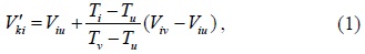
where
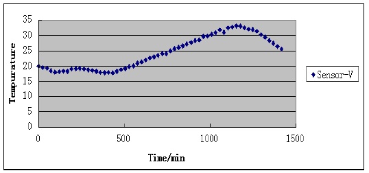
For a single missing data element, the TCA-LI algorithm can give a better attestation value, but if the missed sensor data are continuous, the accuracy of the TCA-LI algorithm decreases, as shown in Fig. 1. Sensor V measures the temperature every 24 minutes. Assuming that
2) TCA-MR Algorithm
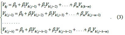
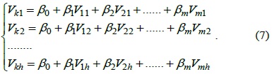
From the above section, we see that TCA-LI has good accuracy for single missing sensor data elements in TCA, but for continuous missing sensor data, TCA-LI cannot provide good estimation data. Therefore, in this section, we will introduce the multiple regression algorithm (TCA-MR) to estimate the continuous missing sensor data of the TCA model. Assuming that

where {
To estimate , we should use the training dataset to estimate the value of {
Let
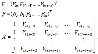
Therefore, Eq. (3) can be rewritten as follows:

The coefficient
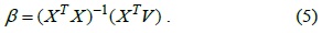
After we calculate the value of coefficient
For continuous missing data and loose temporal correlation parameters, the TCA algorithm cannot provide a good estimation value for the missing data. However, the SCA algorithm can discover the spatial relationship between the sensor nodes and use the discovered spatial knowledge to estimate the missing data.
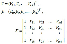
Assuming that

where {
To calculate SCA needs a dataset to estimate the value of {
Let

Therefore, Eq. (3) can be represented by using matrix algebra as follows:
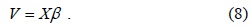
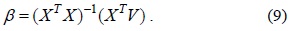
Hence, we can calculate the value of coefficient

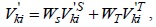
The TCA algorithm is always used for estimating tight temporal correlations and single missing data elements. The SRA algorithm is used for estimating tight spatial correlations. However, when the temporal or spatial correlation is unknown, TCA or SCA may not give a good estimation value. To solve this problem, the STCA algorithm is proposed. This algorithm takes into account the weight of the temporal and spatial correlations; therefore, the STCA algorithm can be represented as follows:

where
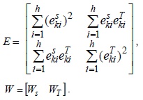
To obtain the optimum value of
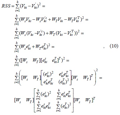
where denote the estimation error of respectively, and
Let

Therefore, this question of getting optimum value of

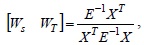
Therefore, we can use the least-squares approach [7] to obtain an optimal solution as follows:

where

>
E. Correlation Analysis Algorithm
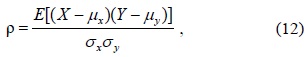
We use Pearson’s product-moment correlation coefficient to measure the correlation of the output variable and the input variable. The value of ρ is between +1 and −1 (inclusive), where 1 denotes a total positive correlation, 0 represents no correlation, and −1 indicates a total negative correlation. The formula for ρ is as follows:

where
Further, 0.5 < |
1) Temporal Correlation Analysis
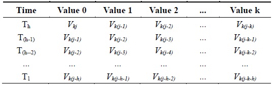
If we want to find whether the sampling data of a sensor have a temporal relationship, we should choose a training dataset for the analysis. Assuming that {
[Table 1.] Dataset at time Th, T(h-1),T(h-2),..., T1

Dataset at time Th, T(h-1),T(h-2),..., T1
Therefore, we can use Eq. (12) to analyze the relationship of the dataset of Th and the dataset of another time (T(h-1),T(h-2),...,T1). Now, we can define the temporal correlation as follows:
Definition 1: In a training dataset, if the sub-dataset of Th is highly relevant to one or more sub-datasets of another time (0.5 < |ρ| ≤ 1), the dataset of the sensor node has a high temporal correlation. If the sub-dataset of Th is only moderately relevant to one or more sub-datasets of another time (0.3 < |ρ| ≤ 0.5), the dataset of the sensor node has a medium temporal correlation.
2) Spatial Correlation Analysis
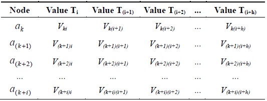
If we want to determine whether the sampling data of a sensor have a spatial relationship, we should also choose a training dataset for the analysis. Assuming that
[Table 2.] Dataset of ak, a(k+1),a(k+2),...,a(k+i) at different times

Dataset of ak, a(k+1),a(k+2),...,a(k+i) at different times
Definition 2: In a training dataset, if the sub-dataset of
>
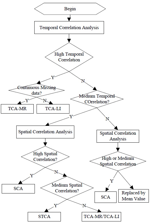
F. Process of STCAM Decision
STCAM uses the following four algorithms: TCA-LI, TCA-MR, SCA, and STCA. If a sensor node has a tight temporal correlation and does not miss continuous data, STCAM will use the TCA-LI or TCA-MR algorithm to estimate the missing sensor data. Further, if a sensor node has a high spatial correlation, STCAM will use SCA to estimate the missing data. Otherwise, STCAM will choose the STCA algorithm. The process of STCAM decision making is shown in Fig. 2. From these figures, we can conclude the applicable conditions of the four algorithms.
TCA-LI: The training dataset has a high temporal correlation when the type of missing sensor data is single. In contrast, the training dataset has a medium temporal correlation when the training dataset has a low spatial correlation and the type of missing sensor data is single.
TCA-MR: The training dataset has a high temporal correlation, and the type of missing sensor data is continuous. The training dataset has a medium temporal correlation when the training dataset has a low spatial correlation and the type of missing sensor data is continuous.
SCA: The training dataset has a medium temporal correlation when the training dataset has a high spatial correlation. The training dataset has a low temporal correlation when the training dataset has a low spatial correlation, and the training dataset has a low temporal correlation when the training dataset has a medium spatial correlation.
STCA: The training dataset has a medium temporal correlation when the training dataset has a medium spatial correlation.
If the training dataset has a low spatial and temporal correlation, there is no matching algorithm for the estimation.
The estimation model proposed in this paper is simulated using Java and evaluated over the Intel lab dataset [8] and a traffic dataset of a city in China. The Intel lab dataset is a trace of readings from 54 sensor nodes deployed in the Intel Research Berkeley lab. These sensor nodes collected the light, humidity, temperature, and voltage readings once every 30 seconds. The traffic dataset is a trace of readings from 596 sensor nodes that are deployed on different roads.
To evaluate the accuracy and performance of STCAM, we choose DESM [9] for a comparison. The DESM algorithm is also an estimation approach based on the spatial-temporal correlation, and the result formula is as follows:

where
To evaluate the four abovementioned algorithms, we need to choose different datasets for testing.
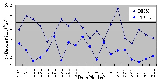
1) Comparison between TCA-LI/TCA-MR and DESM
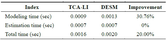
By analyzing the temporal correlation, we know that the temperature dataset has a high temporal correlation; therefore, we use the temperature dataset of sensor 23 to test the accuracy and performance of TCA-LI/TCA-MR. Firstly, we assume that the 121th, 131th, 141th,..., 311th data elements are missed; therefore, under this condition, STCAM chooses the TCA-LI algorithm to estimate the missing sensor data. The experiment results are presented in Fig. 3 and Table 3.
[Table 3.] Performance comparison of TCA-LI and DESM

Performance comparison of TCA-LI and DESM
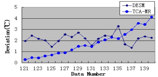
We assume that data 121–140 are missing; therefore, under this condition, STCAM chooses the TCA-MR algorithm to estimate the missing sensor data. The experiment results are presented in Fig. 4 and Table 4.
[Table 4.] Performance comparison of TCA-MR and DESM
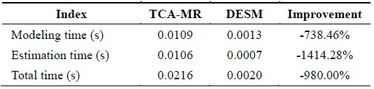
Performance comparison of TCA-MR and DESM
According to Fig. 4, the accuracy of TCA-MR decreases with an increase in the amount of continuous missing sensor data. Therefore, there is a threshold. If the amount of missing sensor data is less than the threshold, TCA-MR exhibits good accuracy, and if the amount of missing sensor data is more than the threshold, TCA-MR is not suitable for estimating the missing sensor data with a high temporal correlation. According to Table 4, the performance of TCA-MR is significantly higher than that of DESM.
2) Comparison between STCA and DESM
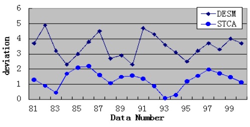
By analyzing the temporal and spatial correlation, we know that the humidity dataset has a medium temporal and spatial correlation. Under this condition, STCAM chooses the STCA algorithm to estimate the missing sensor data. We choose the humidity dataset of sensor 11 to test the accuracy and performance of STCA. Assuming that data 81–105 are missing, we obtain the experimental results shown in Fig. 5 and Table 5.
[Table 5.] Performance comparison of STCA and DESM
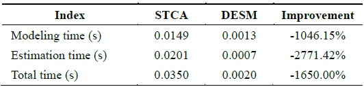
Performance comparison of STCA and DESM
According to Fig. 5 and Table 5, STCA exhibits better accuracy, but the performance is lower than that of DESM.
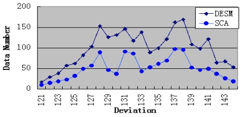
3) Comparison between SCA and DESM
By analyzing the temporal and spatial correlation, we find that the traffic dataset has a low temporal correlation and a high spatial correlation. Therefore, under this condition, STCAM chooses the SCA algorithm to estimate the missing sensor data. We suppose that data 121–144 of sensor
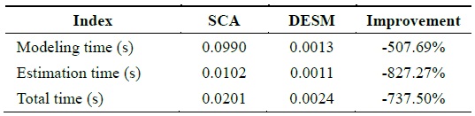
[Table 6.] Performance comparison of SCA and DESM

Performance comparison of SCA and DESM
According to Fig. 6 and Table 6, SCA exhibits better accuracy, but the performance is lower than that of DESM.
In this paper, we propose a data estimation technique called STCAM, which can discover the correlation of the training dataset, and depending on this correlation and the type of missing sensor data, STCAM can choose one of the most suitable algorithms from SCA-LI, SCA-MR, TCA, and STCA to estimate the missing sensor data. From the simulation result, we conclude that STCAM exhibits good accuracy for the missing sensor data, but in terms of performance, STCAM has a relatively low computational efficiency. Therefore, STCAM can only be deployed at the sink node or in the central server. Moreover, by the simulation, we found that the accuracy of TCA-MR decreases with an increase in the amount of continuous missing sensor data, and this may influence the total accuracy of STCAM, but in the paper, we do not provide an effective solution for this issue. Therefore, in the future, we will conduct further research to fill the gap.