Economic growth and prosperity are often taken for granted by those who fortunately live in the richer part of the world. While residents of rich countries reap the positive effects of better health systems, commodities and services, very fewof them can imagine people in less developed countrieswho are suffering from poverty.While factors such as insufficient natural resources, overpopulation, an unstable political environment, and slowtechnological development are known to contribute to the continuing poverty in less developed countries, poor health conditions stand out as the most frightening one.
Economists who study development and growth theory have long recognized the important role of education in the formation of human capital. However, they have not widely acknowledged health as another vital force in the formation of human capital. In this paper, a neoclassical growth model will be utilized to highlight the important role of health in human capital and its ultimate impact on economic well-being.1 We apply longitudinal data (i.e., panel data) analysis to examine how health status contributes to average income differences in the selected countries over time. While similar studies have focused on how health affects economic outcomes such as total output (real GDP), productivity (real GDP per labor input) and GDP growth rate, our paper is different from those in at least three ways. First, we use average income as the dependent variable, which is a better proxy for measuring the richness/poorness of nations. Second, many studies lack appropriate estimators to deal with common autocorrelation and heteroskedascity problems presented in panel data models. We use unrestricted feasible generalized least square (unrestricted FGLS) estimators to overcome these problems. Third, health and other growth factors are endogenous (i.e. reverse causality between the dependent and independent variables) by nature; the existence of a correlation between regressors and error terms may result in biased estimates.We use the instrument variables method to reduce this biasedness.
To make sure the sample covers both high- and low-income economies, we carefully select 52 countries among different income groups based on the World Bank’s GNI (gross national income) per capita information. Whereas the data from past studies all end in 1995 or earlier, we expand the data set to include the most recently available data from2000. By covering countries with various average income levels over longer time horizons in this study, we are able to obtain more representative and efficient estimates for analyzing how health status contributes to income variations and standards of living. The ultimate goal in this paper is to quantify the impact of health on average income. Our main empirical finding indicates that a one-year increase in life expectancy raises GDP per capita by 0.5–0.9%. Consequently, this information can be beneficial to poor countries in achieving a targeted average income level by allocating limited resources to the appropriate health-promoting sectors.
The remainder of the paper is organized as follows. Section 2 contains the literature review. Section 3 introduces a Cobb-Douglas type aggregate production function to illustrate how health and other factors determine the average income in a country. Section 4 describes the data and provides some preliminary descriptive statistics. Section 5 details the empirical models and reports the empirical test results. Section 6 contains a summary and conclusions.
1Economic well-being is represented by ‘average income’, which is measured by ‘GDP per capita’ using international PPP price. We use these two terms interchangeably in this paper. Downloaded by [Yonsei University] at 20:01 24 July 2011
Since the pioneering work of Solow (1956) and Swan (1956), growth theory has evolved into a major economic field. Labor, physical capital, technology, and human capital have been gradually introduced into economic growth models. Mankiw
Nowadays, it is generally agreed that health is one of the most important assets a human being possesses. Healthier workers are more productive; they are physically and mentally stronger and less likely to be absent from their jobs due to illness. Therefore, health should not be excluded as a factor in the formation of human capital. Grossman (1972) develops a health-demand model that introduces the concept of health capital into the literature in his pioneering paper.He explains that healthy people are more production-efficient and consequently contribute to higher labor productivity. Barro (1996) comments that health is a productive asset and an engine of economic growth. Following the Ramsey scheme, he develops an economic growth model that brings in health capital as one of the important growth factors. Observing the vicious cycle of poor health and poverty in Africa, Sala-i-Martin (2006) suggests that government interventions must be aimed at promoting health as the main approach to eradicating poverty; reducing poverty is indispensable to fostering economic growth.
How do we measure health and how does health contribute to economic growth? Researchers who have examined the link between health and economic outcomes, at either the micro (individual) or the macro (national) level, have generally used two types of health measures: inputs into health and health outcomes (Weil, 2007). According toWeil, health inputs refer to the physical factors that influence an individual’s health. These factors include nutrition, available medical care, living environment, and so forth. Health outcomes are determined both by an individual’s health inputs and by his genetic endowment. Examples include life expectancy, height, and ability to work.
A substantial number of micro studies have analyzed how various indicators of health outcomes are positively related to labor income and productivity. Strauss and Thomas (1998) give a comprehensive review of the empirical evidence. In macroeconomic studies, Fogel (1994) was among the first to examine the link between health indicators, the mortality/morbidity rate, and economic growth. His health indicators include height at given ages, weight at given ages, andweight-for-height (i.e. BMI, a body mass index). Barro and Lee (1994) cite the importance of human capital (in the form of both education and health) in the economic growth process. They find that health, measured by life expectancy, has a significant and positive effect on economic growth. However, Barro and Sala-i-Martin (1995) do not find a significant relationship between life expectancy and growth in their cross-country growth regression.
Based on the Solow growth model, Bloom
2In addition to education and health, working experience is another potential candidate for representing human capital (Bloom et al., 2004). Experience data can be collected via survey questions and used in micro studies. However, such data often do not exist in macro (across-country) studies.
3. Health in the Economic Growth Model
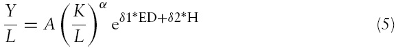
Following the neoclassical approach, we write a Cobb-Douglas type aggregate production function in the spirit of Weil (2007) as:

where

Equation (2) states that human capital consists of education (ED) and health (H) and their relationship is represented by an exponential function4 (exp). Betas are parameters attached to each component of human capital. Substitute equation (2) into equation (1) and we can obtain the following:

After multiplying the parameter 1–

where

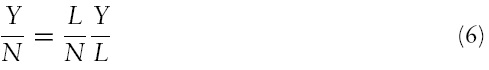
GDP per capita (average income) can be decomposed into a product of laborpopulation ratio and average labor productivity as shown in equation (6), where

We substitute equations (5) into (6) and the final growth equation (7) is shown in the following:
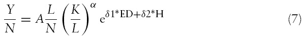
A testable empirical equation based on equation (7) is shown in the following:

where
3In practice, it also includes other factors such as culture, political stability, government policies, etc. 4In section 4, we show that education and health are linearly related to the log of average income.
4. Data Specifications and Descriptive Statistics
The data were collected from different sources. The data set consists of a panel of 52 countries5 observed every 5 years from 1970 to 2000. The total degree of freedom is 364 (52 × 7).RealGDPper capita data (measured in 1996 international purchasing power parity dollars) and national populationwere obtained from the Penn World Tables (Heston
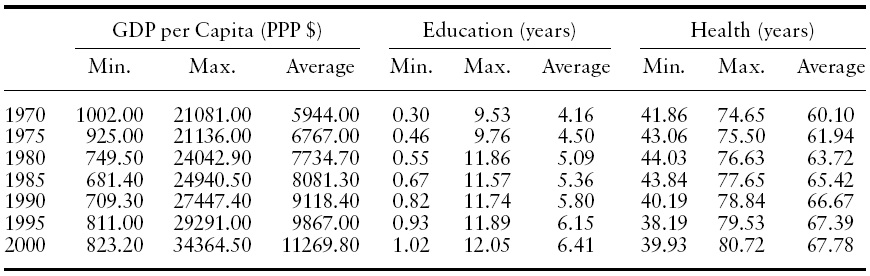
[Table 1.] Descriptive statistics

Descriptive statistics
Labor supply (or labor force) and life expectancy at birth in each country were obtained from the World Bank’s Indicators CD-ROM. The education data were obtained from a study by Barro and Lee (2001), wherein education was measured as the average schooling years of the population over age 15.
While a direct measure of capital is often not available for less developed economies, we use the investment/real GDP ratio obtained from the PennWorld Tables to generate the capital stock as proxy. Following Bloom
Table 1 provides some descriptive statistics that include the minimum, maximum, and average values for GDP per capita, education, and health over seven time periods. The table shows that the average value of GDP per capita and two human capital measurements move in the same direction over time. In 1970, the average income of the richest country (Switzerland) is about 20 times that of the poorest country (Mozambique). In 2000, the average income of the richest country (United States) is 40 times that of the poorest country (Togo). Our data reveal that poor countries have been stuck in the poverty trap. Turning to both human capital components, from1970 to 2000, average schooling years have increased by 54.08% and average life expectancy has increased by 12.78%. According to the data in 2000, a baby born in Japan can expect to live 80 years. However, average life expectancy at birth in Rwanda or Zimbabwe is a mere 40 years (39.93 and 39.94 respectively), half of Japan’s level. One striking fact in the original data also reveals that while the educational level has been increasing at different rates in all 52 countries, life expectancy in poor economies is either stagnant or even decreasing. Based on these figures, we observe that poor health can be a deciding factor that differentiates rich economies from poor ones.
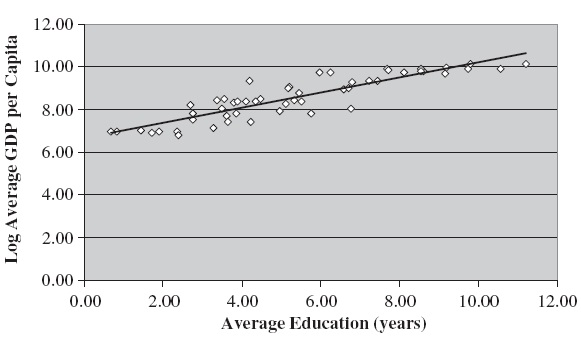
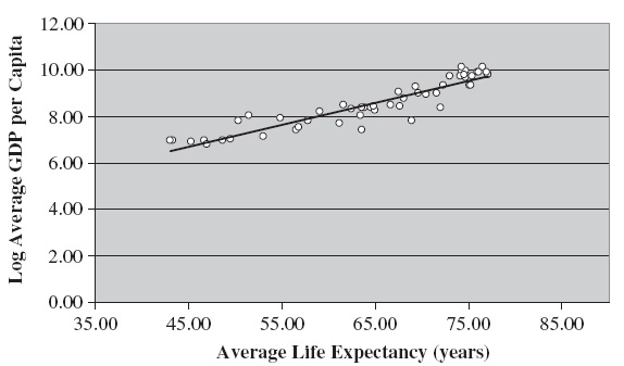
Some micro studies (see Strauss & Thomas, 1998; Card, 2001) often suggest that the log of labor income has a linear relationship with years of education attained and life expectancy. We plot the log of average GDP per capita against a measure of average education (schooling) and average health (life expectancy), respectively. Figures 1 and 2 reveal that both human capital components have linear relationships with the log of GDP per capita (average income).
5Using the World Bank’s Gross National Income (GNI) per capita criteria in 2008, these 52 economies can be divided into ‘High&Upper Middle Income’ and ‘Lower Middle&Low Income’ countries based on average GDP per capita data calculated from our sample. The former countries include Austria, Canada, Chile, Colombia, Cyprus, Denmark, the Dominican Republic, Finland, Greece, Iceland, Italy, Israel, Jamaica, Japan, Malaysia, Mauritius, the Netherlands, Portugal, Singapore, Sweden, Switzerland, Trinidad and Tobago, Turkey, the UK, the US, and Uruguay, Downloaded by [Yonsei University] at 20:01 24 July 2011 Venezuela (27 countries in total). The latter countries include Benin, Bolivia, Cameroon, Central African Republic, Ecuador, El Salvador, Guatemala, Honduras, India, Indonesia, Kenya, Mozambique, Nicaragua, Nigeria, Pakistan, Paraguay, Philippines, Rwanda, Sri Lanka, Syria, Thailand, Togo, Tunisia, Uganda, Zimbabwe (25 countries in total).
5. Empirical Framework and Test Results
We apply three commonly used panel data models, which include pooled, fixed effect, and random effect models, to examine how the economic growth factors specified in equation (8) affect average income in a panel of countries over time. If they do contribute to an increase in GDP per capita, we should expect the estimated coefficient attached to each factor to be statistically significant and have a positive sign. Special attention will be paid to the size of
On the basis of the assumption on the error term,

Equation (9) states that the error termconsists of both systematic (
Using equation (9), we can obtain the following regression equation as:

Equation (10) is termed a linear unobserved effects panel data model. It is very common to have autocorrelation and heteroskedascity present in residuals in the panel data models; we use unrestricted6 FGLS estimators (seeWooldridge, 2002, 10.4.3 and 10.5.5) to solve both problems in order to achieve consistent and more efficient estimates. Although we apply the Hausman (1978) test to choose between the fixed effect and random effect model, results from both are reported for comparison and inference purposes.With regard to the reverse causality problem, average income may affect growth factors. We use lagged growth factors as instruments to achieve orthogonality between regressors and the error term.
Examining the descriptive statistics in Table 1, we find that average GDP per capita, health, and education all contain a time trend. Therefore, it is likely that the empirical results obtained from our panel data models are spurious (Granger & Newbold, 1974). With that in mind, we remove the trend using the differenced method7 and investigate whether the empirical result becomes significantly different. It is well known in the field of public health that data on life expectancy at birth are highly sensitive to the infant mortality rate. The health data used in our empirical study may underestimate life expectancy at birth for less developed economies due to their consistently high infant mortality rates. Using the differenced method can successfully reduce this bias, since the differenced health variable (ΔH) would remain stable.
[Table 2.] Pooled model using FGLS
Pooled model using FGLS
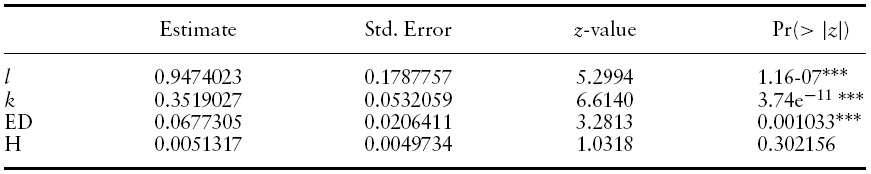
[Table 3.] Fixed effect model using FGLS

Fixed effect model using FGLS
We first run the pool model and the results are reported in Table 2.The statistics indicate that the absence of individual effect is rejected. Therefore, we proceed to test the fixed effect and random effect models. Due to the detection of autocorrelation and heteroskedascity in residuals, we turn to unrestricted FGLS estimators to find unbiased estimates. The results are reported in Tables 3 and 4, respectively.
By comparing these two tables, all of the estimated coefficients appear to carry their expected signs; the labor–population ratio, physical capital–labor ratio, education, and life expectancy all have positive impacts on real GDP per capita. In both models, the estimated parameter for the labor-population ratio is close to one. The t-statistics indicate that all of the estimates are significant at least at the 10% level.
We run the Hausman test8 to decide whether a random or fixed effect model is more appropriate. The null hypothesis in this test is that the individual effect is correlated with the regressors against the alternative hypothesis when they are uncorrelated. The test statistic will be distributed asymptotically as a Chi-square, given that the null hypothesis is true. The test result in Table 5 indicates that there is no correlation between individual effect and regressors, and, therefore, the random effect model seems to be the more appropriate model to adopt. In Table 4, the estimate for the physical capital–labor ratio is about 0.5; we can interpret this to mean that a 1% increase in this ratio raises GDP per capita by 0.5%. If we turn to equation (3) in section 3, this estimate says that 50% of national income (real GDP) is paid to physical capital and the other 50% is paid to efficient labor. This result is similar to the finding in Bloom
[Table 4.] Random effect model using FGLS

Random effect model using FGLS
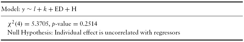
Hausman test 1
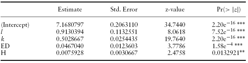
We turn our attention to the estimates of human capital in the formof education and health. The estimates for education and life expectancy are 0.0467 and 0.0076 (rounded to fourth decimal points), respectively. Since both education and life expectancy are measured in years, the estimates indicate that one additional year of education increases average income by 4.67%. On the other hand, raising life expectancy by one year increases average income by 0.76%. Since similar empirical studies have used other economic outcome variables as the dependent variable, we cannot directly compare these estimates. However, they all share the common finding that education and health do have positive effects on economic outcomes (economic growth, labor productivity, or, in our case, average income). Our results further explain why the income gap between rich and poor countries was getting larger and larger during the sample period (1970–2000). While life expectancy in rich countries had gradually increased, life expectancy in poor countries had been either stagnant or even decreasing.
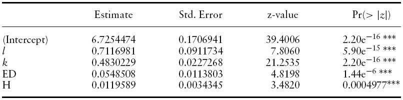
[Table 6.] Fixed effect model using instrument method & FGLS
Fixed effect model using instrument method & FGLS
[Table 7.] Random effect model using instrument method & FGLS
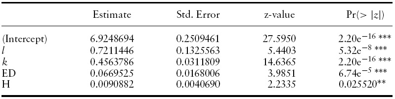
Random effect model using instrument method & FGLS
Reverse causality calls for the use of the instrument variables method.Replacing the regressors with their lagged counterparts,9 we apply the unrestricted FGLS estimator on both fixed effect and random effect models. The results are reported in Tables 6 and 7, respectively. Although the Hausman test result reported in Table 8 indicates that the fixed effect model should be adopted, given that the null hypothesis is rejected,10 we summarize results fromboth models and compare them to the results when reverse causality is ignored.
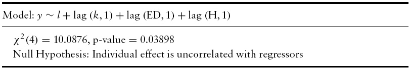
Hausman Test 2
[Table 9.] Model using differenced method & FGLS
Model using differenced method & FGLS
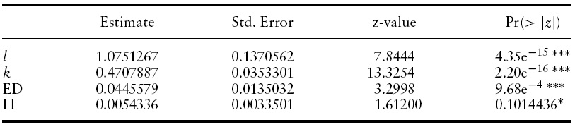
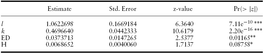
First, all of the estimates carry the expected positive signs. However, the estimate of the health variable is no longer significant in the fixed effect model.
Second, both estimates of human capital components become larger. In other words, their contribution to average income should be stronger when reverse causality is taken into consideration. The impact of education on average income increases from about 4.50% to 6.70% in both fixed and random effect models. The impact of health on average income remains the same (0.5%) in the fixed effect model. However, the impact increases from about 0.76% to 0.90% in the random effect model.
Third, the share of national income paid to physical capital becomes smaller in both the fixed effect and the random effect model. In the fixed (random) effect model, this share drops from 0.47 (0.50) to about 0.35 (0.45). This result is close to the typical finding that about 1/3 of income is paid to physical capital (see Mankiw, 1992).
To determine the potential danger of finding spurious relationships due to the trend variables, we use the differenced method to remove the trend and test our empirical model. Meanwhile, we expect that the differenced method will successfully reduce the bias of the health measurement due to its sensitivity to high infant mortality rates found in most less developed countries. Table 9 shows that all estimates are significant at the 10% level; they all carry the expected signs, similar to earlier findings for the fixed and random effect models. Quantitatively, the estimated coefficients of health and education are close to our prior findings; the estimates indicate that one additional year of education increases average income by 3.74%. On the other hand, raising the life expectancy by one year increases average income by 0.69%. These results suggest that our empirical results are not sensitive to trend variables, and, therefore, the relationships we find are not spurious.
The information obtained from these estimates may help policy makers to allocate resources more efficiently to increase standards of living. For example, knowing that an additional year of schooling raises average income by 6.70%, the government can increase educational spending to achieve a targeted average education level. On the other hand, the positive impact of life expectancy on average income can give policy makers some guidance about how to direct resources to health-care sectors. If an empirical link can be further established between health inputs and life expectancy, the money can be spent more efficiently. For example, a regression can be used to find how life expectancy is affected by the number of physicians, medical beds, pollution factors, dietary habits and so forth.
6The idiosyncratic component (εit) is both heteroskedastic and serially correlated. 7The estimation equation after differencing is Δyit = Δlit + α∗Δkit + δ1∗ΔEDit + δ2∗ΔHit + Δεit, where ‘Δ’ is the difference symbol. For example, Δyit = yit − yit−1. If the estimated coefficients (α, δ1, δ2) are quite different after applying the differencing method, it is likely the results we get from estimating equation (10) are spurious. 8The test is not actually a selection test. It is to compare whether the fixed effect model (estimator) is different from the random effect model (estimator). If the null hypothesis is true, the difference between these two estimators approaches zero asymptotically (see Verbeek, 2004, 10.2.3). 9All of the regressors except for the labor–population ratio are replaced by their first lagged counterparts. The labor–population ratio in each country has been steady over the sample period and so it is unlikely to be affected by average income. 10Although the random effect model is rejected by the Hausman test, we don’t refute its usefulness for inference purposes. The individual specific effect ai in equation (9) can be ‘random’ in nature, considering that our data on 52 countries are a mere sample drawn from the population of more than 200 countries. Frees (2004) explains why both fixed and random effect models are important in practice.
Economists have long searched for remedies thatmay help less developed countries escape persistent poverty. According to Maddison (2001), theGDPper capita ratio of the richest countries to the poorest ones increased from 11 in 1950 to 19 in 1998. This gap represents a severe income inequality and lopsided standard of living between rich and poor countries. Additionally, poor health caused by preventable diseases and disabilities stands out as a possible candidate to explain why these poor countries cannot achieve greater prosperity.
In order to get the right prescription, an accurate and careful diagnosis must first be conducted. In this paper, we use a neoclassical growth model as a foundation to study how health and other factors contribute to average income. Using panel data that include 52 countries over seven time periods, our empirical results indicate that the physical capital–labor ratio and human capital in terms of education and health are crucial factors contributing to the increase in average income. Our results are consistent with the findings in other similar studies, although the economic outcomes used in the dependent variable may be different. In terms of magnitude, our main empirical result indicates that raising life expectancy does have a positive effect on average income. The impact is in the range of 0.5–0.9%, depending on which model is applied and whether reverse causality is taken into consideration.
We seek to exploit our empirical results in order to provide better policy recommendations for less developed economies. Based on our findings, means and channels of distributing limited resources can be built to maximize those factors that contribute to economic growth. Funding priorities can be established that will help to alleviate the vicious cycle of poverty in poor economies. However, at the same time, we need to point out that the size of these estimates can be sensitive to model specifications and violation of model assumptions. For example, the implementation of the instrument method lowers the share of national income paid to physical capital, and, at the same time, the magnitude of both human capital components increases. Based on these estimates of sensitivity, our future research will be aimed at how to get more robust estimates by using advanced panel data approaches. Hopefully, this study provides useful information to policy makers in their efforts to promote increased economic well-being.