Trade has always been the raison d’être for Singapore’s existence as a political entity – first as a colony of the British Empire, and then as an independent nation-state. The economic historian Wong Lin Ken (2003) has documented how Singapore’s commercial growth in the early nineteenth century depended on the expansion of trade with countries in the Malay Archipelago. By the time the Suez Canal opened in 1869, Singapore’s lifeblood was the entrepôt trade in natural produce and consumer goods between Europe and Asia that was conducted through her free port. During the first half of the twentieth century, Singapore took on the role of a staple port, processing and re-exporting the tin and rubber imported from Malaya and Dutch East India (Huff, 1994).

Despite the unsuccessful merger with Malaysia and political independence in 1965, re-exports continued to grow such that they still accounted for half of total trade in 2007, which itself multiplied to three times the value of domestic output. As Singapore’s neighbors moved away from being primary commodity producers to become manufacturing powerhouses during the 1990s, however, the entrepôt trade in agricultural and mineral products gave way to re-exports of machinery and equipment, particularly electronic components.Re-exports of oil and exports of petrochemicals also became more prominent as a result of increased storage and refining facilities on the offshore islands of Singapore.

Partly on account of her sustained role as the entrepôt for Southeast Asia, modern Singapore has been called a ‘re-export economy’ by Lloyd and Sandilands (1986). But the more cogent reason for the label is the widespread engagement from 1965 onwards of multinational corporations, or their subsidiaries, in activities involving the importation of raw materials and their transformation into domestic exports – manufactures that have been subject to a greater degree of local processing than just repackaging and transhipment – destined for regional or world markets. In the early stage of industrialization, such ‘re-exports’ mainly took the form of garments and cheap electronics. Over the years, however, the product composition shifted to progressively higher value-added goods owing to changing comparative advantages and official efforts to restructure the economy. During the 1990s, for example, the share in domestic exports of sophisticated electronic products such as disk drives, computer peripherals, and integrated circuits rose to nearly 70% as the global semiconductor market boomed. Nonetheless, the proportion of import content in gross value-added remains high as a result of production fragmentation and the vertical integration of the regional supply chain based in Asia.

This article revisits the hypothesis that Singapore is a re-export economy in modern guise. Rather than follow Lloyd & Sandilands’ strategy of netting out the direct and indirect imported inputs used in the production of domestic exports to derive a measure of local value-added, the investigation here applies time series econometric techniques. If the hypothesis is true, there would be a natural tendency for merchandize exports and imports to co-move together over the course of cyclical fluctuations induced by foreign demand shocks. The hypothesis also implies that both domestic and pure entrepôt exports are relatively insensitive to exchange rate changes due to their high import content or, stated differently, low domestic value-added. In particular, an appreciating currency would raise Singapore’s export prices in world markets but at the same time reduce the domestic costs of imported raw materials, thus leaving price competitiveness essentially unaltered.

To test these empirical implications of the re-export economy hypothesis for the joint behavior of Singapore’s trade aggregates, a structural vector error correction model (SVECM) that includes proxies for external demand and relative prices is specified in Section 2. In Section 3, the choice of this model is justified by unit root and cointegration tests with structural breaks. Section 4 estimates theVECM, identifies the structural shocks in the model through short and long-run economic restrictions, and analyzes the dynamic reactions of the trade variables to demand and price shocks by means of impulse responses and variance decompositions. In Section 5, the evidence is brought to bear on the validity of the re-export economy hypothesis for Singapore and its policy implications are contrasted with the case of conventional economies.

The empirical study of trade between countries has a long and well-established tradition in applied international economics.Asurvey of the large literature based on the ‘standard trade model’ reveals that the most popular approach used in econometric analysis revolved around the estimation of structural demand and/or supply functions relating exports (or imports) to relevant income and relative price variables.1 Moreover, the majority of published studies have executed this strategy in a single rather than simultaneous equation framework.

Recent work has emphasized instead the non-stationarities in the foreign trade data and accordingly estimated cointegrating relationships in the long run and error-correction models in the short run. Abeysinghe and Choy (2007) provides a good example of this methodology in the case of Singapore. They first derived a theoretical model of exports that allows both demand and supply factors to determine trade flows. This model is then used as a guide to the estimation of export equations for different categories of traded goods, which constitute part of a larger macroeconometric model of the Singapore economy.

Amultivariate analogue of these equations is the vector error correction model (VECM) given by:

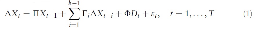
where

is a vector of first-differenced time series, D_t contains deterministic terms with coefficient matrix Φ, and ∏ and Г_i are 6 × 6 matrices of unobserved parameters. The innovations εt are assumed to be i.i.d. Gaussian processes with

In the model, foreign output (f_t ) serves as a proxy for general external demand while worldwide semiconductor sales (s_t ) is an excellent indicator of global electronics demand. Given Singapore’s heavy reliance on the electronics trade, as mentioned in the introduction, the inclusion of the latter variable is essential. On the supply side, a measure of the real effective exchange rate (e_t ) is used to capture the potential impact of relative price and currency movements on the country’s cost competitiveness.2 The trade aggregates included in the model are domestic exports (x_t ), re-exports (r_t ) and imports (m_t), the last consisting predominantly of re-export goods and intermediate inputs.

If the individual series are integrated of the first-order and also jointly cointegrated, then rank(∏) = r < 6 and (∏) can be reconstituted as the outer product αβ’, where α and β are 6 × r full rank matrices and r is the number of cointegrating relations present in the model. The columns of β are the coefficients of the cointegration vectors and the rows of α are the loadings on the errorcorrection term β’X_t-1 in each equation. Hansen (2005) has recently shown that under mild conditions, the VECM in equation (1) has the closed-form representation:

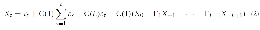
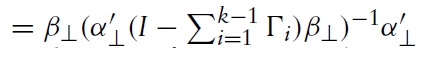
in which C(1)

and the subscript ⊥ denotes the orthogonal complement of a matrix. The coefficients of the lag polynomial C(L) are given by a set of Yule-Walker equations while the precise form of the deterministic term τ_t depends on D_t.

Equation (2) can be viewed as the multivariate Beveridge-Nelson decomposition of the endogenous variables into a deterministic time trend; common stochastic trends (or permanent shocks); and stationary cycles (or transitory disturbances), subject to the initial values given by X₀,X₋₁, . . . ,X_−k+1. In the next section, cointegration is tested and it is found that r = 3, suggesting the existence of three stationary relations in the model and the same number of transitory shocks. The corollary is that there are only 6 − r = 3 shocks that can have permanent effects on the variables of the system. For a small open economy, it is reasonable to postulate that the permanent shocks are those associated with global output fluctuations, electronics disturbances and real exchange rate movements, since these are the putative causes of Singapore’s trade cycles.

Making the further assumption that the permanent and transitory shocks are orthogonal to each other enables the model to be partially identified and converts it into a structural VECM. The idea is to transform the C(1) matrix into A(1) and C(L) correspondingly into A(L) (see King et al., 1991). The elements of the A(1) matrix measures the long-run impact of the common trends on individual variables, while A(L) contains the dynamic effects of the permanent and transitory perturbations. Since C(1) is a reduced rank matrix, the zero columns in A(1), which ensure that transitory shocks have no long-run effects, provide only 3 × r = 9 independent restrictions. To exactly identify the permanent shocks, another 3(3 − 1)/2 = 3 restrictions are imposed on the first three columns of the contemporaneous A₀ matrix as follows3 (A₀ is the first entry in A(L)):

In words, shocks to semiconductor sales are not allowed to have any immediate impact on foreign output, while domestic real exchange rate disturbances do not affect global variables. The first restriction is based on the premise that it is world production that drives electronics spending in the short term, and not the other way round, even though electronics fluctuations may well have medium-run effects on foreign output. The second and third constraints essentially state that shocks originating from Singapore cannot have any effect on the rest of theworld. In contrast, international disturbances and changes in price competitiveness can have contemporaneous effects on the domestic trade aggregates.

1Strauß (2004) contains a detailed review of the standard model and the applied literature.  2Another variable that is occasionally included in export supply equations is the economy’s production capacity.However, the absence of a capital stock time series in Singapore and the unsatisfactory nature of the perpetual inventory method for constructing one, especially at the monthly frequency, meant that this variable had to be left out of the empirical analysis.  3The article’s focus is on the permanent shocks as identification of the transitory disturbances is not necessary for testing the re-export economy hypothesis.

Taking off from where Lloyd and Sandilands (1986) terminated their study, monthly data beginning from 1990 and ending in 2007 is analyzed. As such, preliminary seasonal adjustments were performed where needed and variables are measured on a logarithmic scale to avoid heteroscedastic effects in trade. The index of foreign output is computed as the export-weighted average of the indices of industrial production in Singapore’s major trading counterparts.4 To obtain a proxy for real electronics demand, the nominal value of global chip sales was downloaded from the Semiconductor Industry Association website and deflated by theUSproducer price index for electronic components and accessories, retrieved from the Bureau of Labor Statistics database (the series identification code is WPU1178). The real effective exchange rate used is from the International Financial Statistics online database.5

The Singapore merchandize trade data in local dollar terms is courtesy of International Enterprise Singapore, the government agency tasked with trade promotion. Unlike the series published by the statistical authority, these customs figures do not include trade with Indonesia.6 Since the oil trade is affected by a different set of factors, it is excluded from the empirical analysis. Therefore, domestic exports, re-exports and imports of only non-oil productswere converted into constant 2006 prices by deflating them with their respective price indices. Had data on intermediate goods imports been available, they would have been used in place of total imports, but this was not the case. Nevertheless, the proportion of imports retained for final consumption pales in comparison with that employed as production inputs.

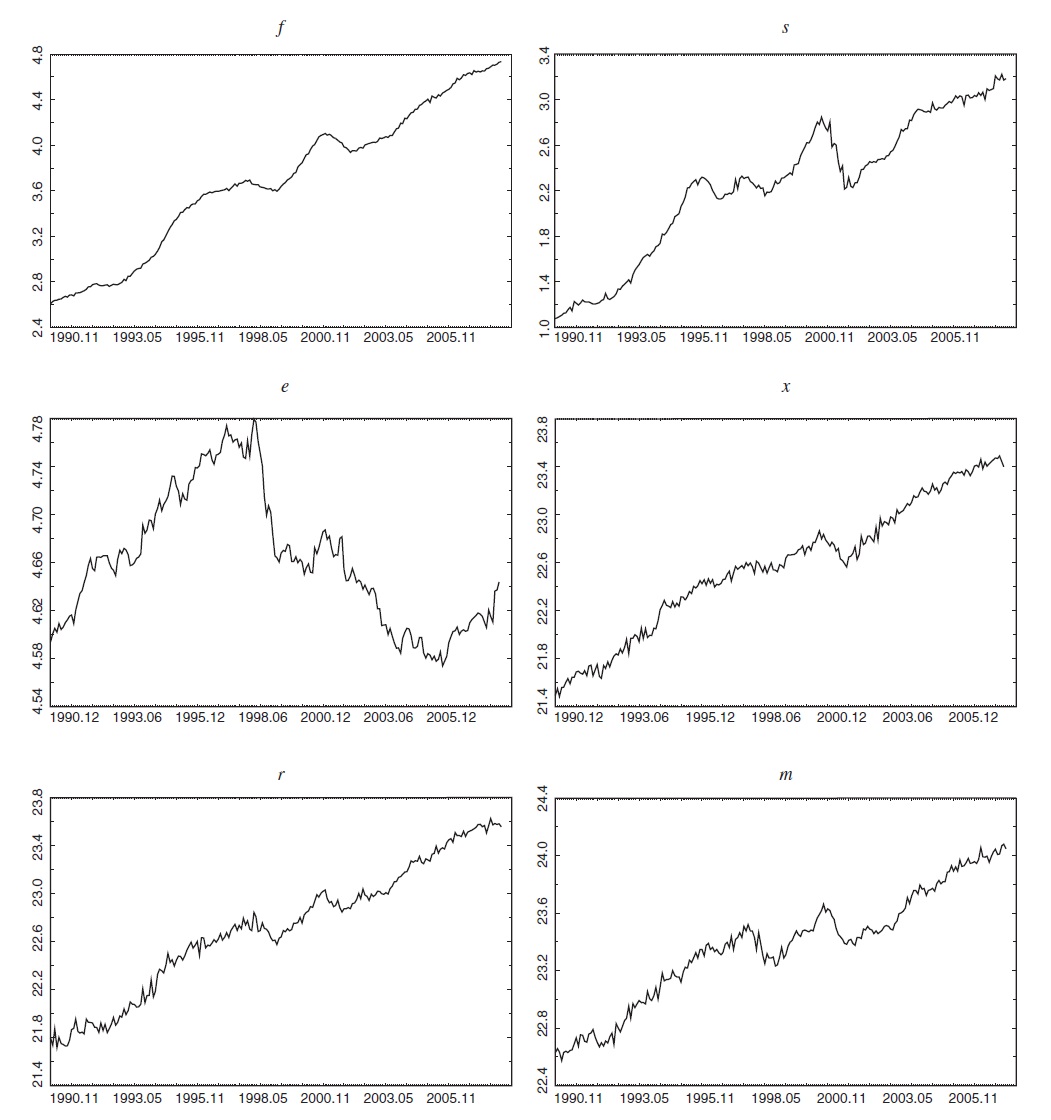
The time series of the above variables are plotted in Figure 1. The proxies for world demand in the first two diagrams exhibit strong upward trends with evident cyclical fluctuations. In contrast, the real exchange rate behaves like a typical random walk characterized by weak mean reversion. Trade cycles are also apparent in the more volatile export and import data, but whether these fluctuations are stationary deviations from deterministic trends or are synonymous with stochastic trends is hard to tell simply by graphic inspection, thus making it necessary to test for unit roots formally.7

In testing for the order of integration of the time series variables, one would notice from Figure 1 that most of them experienced a downward shift some time in late 2000 due to the collapse of global electronics demand upon the bursting of the information technology bubble. This structural break is most conspicuous in semiconductor sales and the Singapore trade series although it is also apparent in foreign industrial production. Consequently, two versions of the augmented Dickey-Fuller (ADF) unit root test are implemented: one without accounting for the structural break and the other after taking it into consideration.

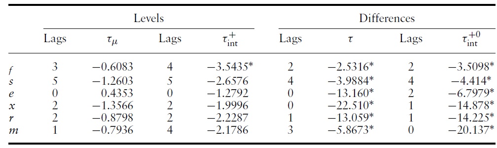
Table 1 reports the results of both types of tests on the logarithmic time series with the number of lags selected by the Hannan-Quinn criterion (HQ), subject to a maximum of 12 months. The standard ADF test statistics with a constant term (τμ) turned out to be insignificant at the conventional level of 5% for every variable.8 Similar tests on the first differences of the variables without the intercept (τ) confirm that they are all difference-stationary.

The second unit root test explicitly allows for a level shift in the series at a known date and is based on Lanne et al. (2002). In this test, the deterministic components of the data generation process, which include a linear time trend and a shift function, are first estimated by a generalized least squares (GLS) procedure. Then the deterministic part is subtracted from the original series and an ADFtype test is applied to the resultant series, in the process correcting for estimation errors in the nuisance parameters.9

The break date is chosen to be December 2000 because thiswas the monthwhen a majority of the time series reached a peak.10 As for the shift function, a step dummy variablewas employed for the test in levels and an impulse dummy for the one in differences – more complicated functions may actually reduce their power. Except for foreign production where the null hypothesis of non-stationarity can only be maintained at the 1% level of significance, the presence of a single unit root in the other series is not rejected by the break tests, as the columns labeled

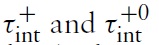
in Table 1 show. The KPSS test, however, rejected trend-stationarity for the former at the 1% level, so it will also be treated as an I(1) variable in what follows.

Returning to Figure 1, it is seen that the Singapore variables co-move with each other, and with global output and chip sales, which provides tentative evidence of cointegrating relationships.Within the bounds of sampling error, these relations can be detected in the multiple cointegration framework of Johansen (1988). His method estimates the ∏ matrix in the VECM of equation (1) consistently by a maximum likelihood (ML) procedure, and then tests its rank with a likelihood ratio trace statistic.

In view of the trending character of the variables in the dataset (save for the exchange rate), an unrestricted constant is included in the deterministic part of the VECM and theHQcriterion was used once more to select a lag length of one. Table 2 presents the outcomes of two different Johansen tests together with their asymptotic critical values. As in the unit root tests, the first ignores the presence of structural breaks. Here, the trace statistics exceed the 95% and 90% quantiles for r ≤ 2, but not those for r ≤ 3, thus indicating that there exists three stationary relations amongst the six integrated variables.

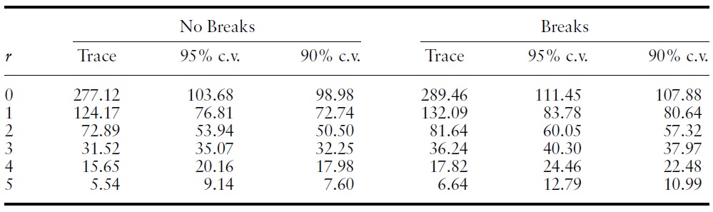
In the second rank test, level shifts in the variables are incorporated into the VECM to coincide with the electronics bust in December 2000. The critical values for this test, as simulated by Johansen et al. (2000) and reproduced in Table 2, confirm that there are still three cointegration vectors to be found between the endogenous variables even when structural breaks are taken into account. These findings therefore strongly suggest that Singapore’s trade aggregates are collectively driven by three transitory shocks and an equal number of common stochastic trends. Following the earlier discussion, the latter are assumed to be synonymous with the permanent shocks in the foreign output, electronics and exchange rate equations.

4These are the US, EU, Japan, Korea, Taiwan, Malaysia, Thailand and India.  5A few missing values in 2003 and 2004 were interpolated using a cubic spline.  6Singapore’s bilateral trade statistics with its close neighbor has been suppressed since preindependence days up till 2003. The official series therefore contains a break, with the data prior to this date excluding this trade and the post-2003 observations including it.  7Incidentally, trade cycles is the old name given to Juglar business cycles with periods of roughly seven years. Here, the term is used more generally to refer to short-run fluctuations in trade aggregates.  8Since the real exchange rate does not exhibit any obvious trend, the constant is omitted in that case.  9The quantiles of the non-standard distribution to which the test statistic converges have been packaged into JMulTi 4.23, the Java interface for theGAUSS routines used to performthe empirical analyses in this paper.  10Lütkepohl and Krätzig (2004) state that the exact location of the break date is not critical as long as it is not totally unreasonable.

The purpose of the current section is to econometrically test the re-export economy hypothesis for Singapore with two standard analytical tools of multivariate time series models – the impulse response functions and innovation accounts backed out from the structural form of the moving average representation in equation (2). Towards this end, the estimation of the SVECM is first addressed.

The SVECM is estimated by a two-step procedure that is equivalent to ML estimation in large samples. In the first step, the parameters of the unrestricted model in equation (1) are obtained by ordinary least squares (OLS) techniques. Initially, ∏ = αβ’, is partitioned as[∏₁ : ∏₂] and β is normalized as [I₃ : β₀]’ to give ∏₁ = α and ∏₂ = αβ’₀. Then the full rank OLS estimator of ∏, denoted

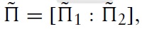
is arrived at by running a regression on each equation after eliminating the shortrun dynamics and deterministic terms, the latter consisting of an intercept and an impulse dummy variable to capture the structural break mentioned earlier. Next, the estimate of β₀ is computed as

where

is the residual covariance matrix. Finally, ΔX_t is regressed on D_t, [I₃ : β₀]X_t−1 and three lags of ΔX_t-i.11

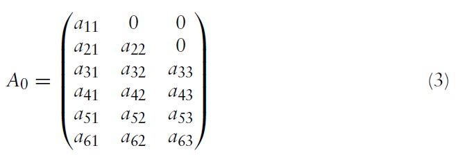
In the second step, the revised estimates of Σ resulting from these regressions are used in conjunction with the long-run restrictions imposed in equation (3) to recover the structural shocks underlying the SVECM. A scoring algorithm is employed in this connection to maximize the concentrated likelihood function, yielding estimates of the A(1) and A(L) matrices that are both asymptotically efficient and normally distributed (see Lütkepohl & Krätzig, 2004 for further technical details).

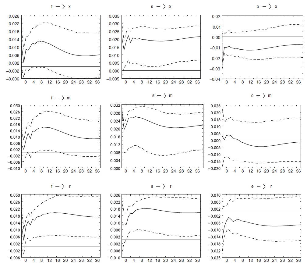
Figure 2 depicts the impulse responses of the levels of x, r and m to the permanent shocks associated with f, s and e. The dashed lines calibrate the estimation uncertainty surrounding the most probable response in the form of 95 percentile confidence intervals derived frombootstrapping theSVECM.12While the abscissa marks the number of months after a unit impulse of one standard deviation has occurred, the ordinate measures the response of a variable in logarithmic units.

The first column of charts show that an increase in foreign output immediately stimulates Singapore’s domestic exports, re-exports and imports in roughly equal measure.This is followed by a temporary dip in trade before the variables converge erratically to their new equilibrium levels after about three years, wherein reexports rise more than the rest. However, the bootstrap confidence bands imply that the impact of an external demand shock on Singapore’s trade volumes is statistically significant only for re-exports in the long run.

In the middle column, a positive shock to the global demand for semiconductors raises the levels of the trade aggregates significantly as well as permanently. There is greater uncertainty encountered at the lower rather than upper bounds of the error bands around the responses. These results are not surprising in view of Singapore’s status as a key electronics producer and her large entrepôt trade in accessories and components. They also suggest that the common stochastic trend in electronics demand is the proximate cause of the unit roots found in the trade series.

The impulse response functions plotted in the last column of Figure 2 show that an unexpected increase in the relative prices of domestic vis-à-vis foreign goods have negative but statistically insignificant effects on domestic exports, reexports and imports. Nonetheless a real currency appreciation does lower exports slightly in the long run due to a loss of competitiveness, although as the re-export economy hypothesis predicts, it has no permanent effect on entrepôt exports, whose impulse response creeps very near to the horizontal axis. Finally, imports decline in tandem with falling exports.

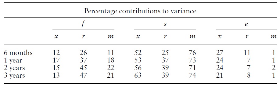
The second set of results obtained from the SVECM provides information on the sources of growth and fluctuations in Singapore’s trade through innovation accounting. As the name suggests, this involves a decomposition of each trade variable’s forecast error variance at future horizons into separate components accounted for by different shocks. Since these are uncorrelated, the error variances are uniquely distributed amongst them in away that reflects the main disturbances influencing the observed movements in the variable.

The variance decompositions of x, r and m due to the permanent shocks are shown in Table 3 for short-termhorizons of six and 12 months and, thereafter, for longer intervals of two to three years. Several regularities stand out. First, global electronics shocks are responsible for the bulk of export and import fluctuations in the short run, confirming the critical roles played by the semiconductor industry and imported inputs in the Singapore economy. Second, these shocks are also a major source of re-export fluctuations, together with foreign demand disturbances. Third, consistent with the impulse responses, re-exports are relatively insensitive to exchange rate perturbations, which account for less than 10% of their fluctuations at most time horizons.

In the long run, semiconductor demand growth continues to power trade flows. Two-thirds to three-quarters of the secular expansion in exports and imports can be traced to the chip industry. Furthermore, foreign production shocks are also important for explaining Singapore’s re-export growth as they contribute nearly half of the forecast error variance at the 2–3 years horizons.

11The additional lags are to ensure that the residuals of the model behave likewhite noise. Moreover, they do not exhibit any signs of autoregressive conditional heteroskedasticity and the Jarque-Bera normality test was passed for all the series except semiconductor sales.  12A non-parametric bootstrap based on re-sampling the residuals 1000 times with replacement was used.

Lloyd and Sandilands (1986) hypothesized that, despite being highly industrialized, modern Singapore remains essentially as a ‘re-export economy’. By that, they meant her trade-driven economy continues to be extremely dependent on imported inputs to satisfy foreign demand. Their provocative claim has the following testable implication in the first instance: exports, re-exports and imports will react in similar fashion when the economy is hit by external demand shocks.

This article sets out to test the re-export hypothesis in a rigorous manner by estimating, identifying and analyzing a multivariate error correction model. Unit root and cointegration tests with structural breaks revealed that such a choice of modeling framework is appropriate for the task. The impulse response patterns yielded by the model demonstrate the existence of ‘trade cycles’ in Singapore, whereby exports, re-exports and imports moved in sync in the short run, hence supporting the main prediction of the re-export economy hypothesis.

A further decomposition of forecast error variances shows that the common stochastic trends behind trade flows explained not only their long-run behavior but also their short-term fluctuations. From an innovation accounting perspective, world semiconductor industry growth was found to be the most important determinant of the trends and cycles in Singapore’s merchandize trade over the last two decades.

The second implication of the re-export economy hypothesis is the insensitivity of domestic and entrepôt exports to exchange rate movements as a result of their high import content. This too has been verified by the empirical analyses here, which suggest that price competitiveness has played only a negligible role in Singapore’s impressive export performance. Indeed, the findings shed newlight on previous research showing that the real exchange rate does not have a significant impact on the trade balance, not just for Singapore but in the case of Malaysia as well – another very open economy in Asia that relies critically on imported inputs for export production (Wilson, 2001). In contrast, Korea’s trade data was found to be consistent with the presence of some ‘J-curve’ effects.

More generally, it is instructive to compare the above feature of a re-export economy with the effects of exchange rate changes in conventional economies that are better endowed with resources. By estimating single equations, Hooper et al. (2000) were able to conclude that export and import volumes in most G-7 industrial countries were responsive to relative price changes, with elasticities ranging from−0.3 to−1.6. One of the exceptions in their study, German exports, were reported also to be sensitive to the real effective exchange rate by Strauß (2004), who took the 1990 reunification into account. The implication for policymakers in these countries is that a real depreciation of the domestic currency would help to reduce an external trade deficit. Conversely, however, exchange rate realignments in a re-export economy such as Singapore will not be an effective means of bringing about internal and external balance in the long run.