This paper analyzes a process bywhich a market boom brought on by a temporary increase in the flow of buyers, can subsequently lead to a collapse of liquidity (speed of sale), prices and production to levels lower than before the onset of the boom. Such episodes accompany a gradual decline in the stock of goods in the market, subsequent to increases in stocks and prices that had occurred at the onset of the boom. Following Krugman (1999), these collective observations are referred to as a hangover effect.1

I consider a general model of markets subject to search frictions in the matching of buyers and sellers. Innovations to the market are deterministic, and agents have perfect foresight.The entry of buyers, and the entry of sellers (through production of new goods) in the market are subject to adjustment costs. These adjustment costs capture a fact that changes in the stocks of buyers and sellers cannot occur at an infinite rate, and allow us to analyze outcomes when there are changes to the flows of buyers and sellers in a market.

In this setting, an exogenous and temporary increase in the entry rate of buyers initially causes liquidity, prices and production to overshoot from its steady state levels due to a positive feedback loop between liquidity and the measure of buyers and sellers. This occurs because liquidity is increasing in the relative measure of buyers to sellers, and higher liquidity increases the measure of buyers, and reduces the measure of sellers, which increase liquidity. Meanwhile, a higher relative measure of buyers to sellers raises prices in favor of sellers, and induces higher production. Thus, during this boom phase there is an expansion of the stock of goods.

As liquidity peaks and then converges down to its steady state level, the stock of goods being sold (and resold in the case of durable goods) remains large relative to its steady state level. The necessary fall of production is signaled through a fall in liquidity and prices (through a fall in the relative measure of buyers to sellers) to below steady state levels. This is the hangover phase. Finally, as the stock of goods converges to its steady state level through lower production and a gradual depreciation of goods, liquidity, prices and production converge toward their steady state levels from below.

A reinterpretation of the canonical Ԛ theory of investment can also generate such cycles in prices and production following a temporary increase in the demand for (durable) goods.2 What differentiates the analysis of this paper from such a model is the link between prices and production with liquidity. Liquidity determines the share of the stock of goods that is up for sale (or unemployment rate), the stock of never sold goods (inventories), and the ratio of the flow of sales to the stock of inventories. A target of the analysis is the set of stylized facts about the correlation of these variables with production, as documented by Blinder and Maccini (1991) and Bils and Kahn (2000) among others.3

An existing search-theoretic literature applied to asset markets includes Duffie et al. (2005), Gârleanu (2006), Lagos and Rocheteau (2007), Miao (2006), Rust and Hall (2003), Spulber (1996), and Weill (2007). An extensive search theoretic literature has been applied to labor markets as summarized in Pissarides (2000). I adopt the framework of Kim (2008), who shows that the canonical search model of unemployment of Pissarides can be modified to consider goods markets subject to search frictions. Differentiating features of this paper are the analysis of out of steady state dynamics when buyer and producer entry rates are subject to adjustment cost.4

In a related paper, Kim (2009) discusses outcomes when the stock of goods is fixed. Here I allow for this stock to be determined endogenously through production of new goods which is a necessary ingredient to generate hangover effects. Related and differentiating results are detailed in the text.

The next section presents the model of markets with search frictions. Section 3 characterizes the dynamics of buyers, sellers and the stock of goods and discusses the hangover effect. Section 4 discusses welfare implications, and Section 5 discusses the rental market. The final section concludes.

1Krugman (1999) defines hangover theory as the view that recessions are a deserved, indeed necessary punishment for previous excesses.  2Reinterpret capital as the stock of good, investment as production of new goods, Ԛ as the price of the good, and rental price of capital as the rental price of the good. Adjustment cost of investment is then an adjustment cost of production. See Romer (2006) for a textbook treatment of the Ԛ-theory of investment.  3These are a countercyclical unemployment rate, procyclical inventory stock and procyclical sales/inventory ratio.  4The counterpart to the entry of buyers and sellers in the labor market model is the entry of job vacancies and unemployed workers. Adjustments costs to the entry of vacancies or unemployed workers have not been considered in the literature. A recent exception is Fujita and Ramey (2007) who consider adjustment costs of vacancies and linearize the dynamics of vacancies and unemployment around the steady state. In contrast, I emphasize the divergent and non-linear dynamics around the steady state implied by such a setting. Blanchard and Diamond (1989) have considered a flow approach to the entry of vacancies in related environments. However, their analysis did not explore the implications of the transition dynamics of market tightness (determining liquidity) which is the focus of my analysis.

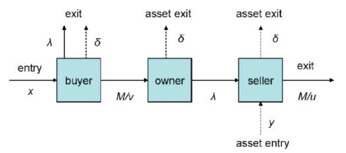
There is a market in continuous time, populated by three types of risk neutral agents who discount at constant rate r: buyers, owners and sellers. Each agent can only hold at most one good in the market. Let v ≥ 0 denote the stock of buyers, s ≥ 0 denote the stock of sellers, and

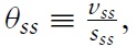
denote their ratio, which we label the tightness of the market. The flow of buyer-seller matches in the market is M ≡ M(v, s) where M_v > 0, M_u ≥ 0, and M is a constant returns to scale function of v, s. Let

denote the rate at which a good is sold, or its liquidity. Let q ≥ s denote the stock of goods in the market, such that q − s denotes the stock of owners. The initial stocks of v₀, s₀, q₀are given.

A buyer of a good searches for a seller and assesses the earnings of the good at π > 0, but with arrival rate λ ≥ 0 reassesses the earnings at πz, z ∈ [0, 1) forever, and exits the market. With arrival rate δ, buyers also assess that the potential good in the market for which they have high valuation depreciates such that they exit the market. The incidence of a match with a seller at rate m(θ)/θ, leads to purchase at sales price P, and change in status from potential buyer to owner.

For an owner, the arrival of the earnings reassessment shock, at rate λ, leads to a change in status from owner to seller, with sales occurring at arrival rate m(θ) at sales price P, after which he exits the market. Owners and sellers also experience depreciation shocks at rate δ ≥ 0, which implies both the good and owner exit the market.5

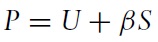
Value equations (or Bellman equations) for buyers V, owners J, sellers U and the sales price P are given by

The flow value of buyers rV, consists of the option value of realizing a match

plus the option value of a reassessment shock −λV, plus the option value of depreciation −δV, plus the capital gains

The flow value of owners rJ, consists of the assessed earnings flow π, plus the option value of a reassessment shock −λ(J − U), plus the option value of depreciation −δJ, plus the capital gains

The flow value of sellers rU, consists of the assessed earnings flow πz, the option value of realizing a match m(θ)(P − U), plus the option value of depreciation −δU, plus the capital gains

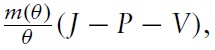
The surplus of a buyer-seller match is S ≡ J − U − V. Let β ∈ [0, 1] denote the exogenous bargaining power of sellers. Sales prices are determined through Nash Bargaining such that

Given the path of

only (determined below), equations (asset) and (nb) specify the values V, J, U, P and S.

Entry into the pool of buyers is determined as follows. New buyers enter the market at rate x(V) > 0where this buyer entry function satisfies x(0) = 0, x’ ≥ 0. Gross entry into the stock of goods is determined as follows. New goods are sourced from production, and enter the market as new sellers at value U. The producer supply curve determines the flow of new goods as a function of this value, y(U) ≥ 0 where y(0) = 0, y’ ≥ 0. Figure 1 summarizes the movement of agents and goods through the market.

This completes the specification of the market. Market specific characteristics are summarized by {λ, δ,m(θ), π, πz, x(V), y(U)}. By varying parameters,we can consider any goods market ranging from consumption goods (low λ, high δ) to durable goods (high λ, low δ) to financial assets (high λ, low δ, high m(θ)). In numerical applicationswhich follow, I consider various markets. In the discussion of rental markets of Section 5, I demonstrate how the analysis maps unto markets where goods are rented out for use rather than through transfer of ownership, such as in the factor market for labor.

It is useful for the analysis to followto characterize values in steady stateswhere

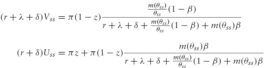
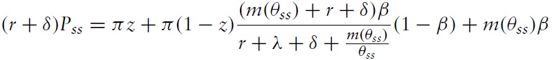
In steady states, the value of the match surplus is

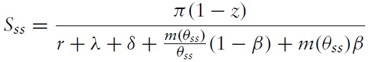
Then, the steady state value of a buyer and seller are respectively given by

Thus, V_ss is monotonically falling in θ_ss, and U_ss is monotonically rising in θ_ss. Both are falling in r, λ, δ, and rising in π. V_ss is falling in z, β, and U_ss is rising in z, β. Lastly, the steady state sales price given by

is monotonically rising in θ_ss. It is falling in r, λ, δ, and rising in π, z, β.6

55In financial markets, where we observe actual earnings, one can think of potential buyers and owners as being optimists and sellers as pessimists, with the actual (average) earnings stream lying somewhere between π and πz. Alternatively, the gap can be interpreted as a holding cost as in Duffie et al. (2005). Downloaded by  6An important point emphasized in Kim (2009) is that the dependence of values on tightness θ, does not depend on the presence of large search frictions. In particular, setting m(θ)→∞implies

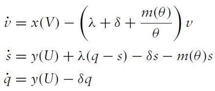
To complete the characterization of outcomes, we need to determine the paths of v, s, q. From the structure of the market detailed above, the dynamics of v, s, q are given by

where the initial v₀, s₀, q₀, are given. The evolution of buyers consists of gross entry of new buyers minus gross exit of buyer through reassessment shocks, depreciation shocks and matches. The evolution of sellers consists of entry of new goods, separation of existing matched goods minus gross exit through depreciation shocks and matches. The evolution of the stock of goods consists of the gross entry of new goods minus the depreciation of existing goods.

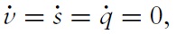
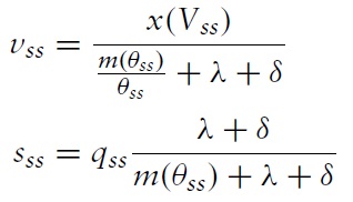
We begin with a characterization of steady state outcomes. In steady states, setting

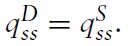
the stock of buyers and the stock of sellers are determined by

The stock of buyers is monotonically increasing in market tightness θ_ss, and the stock of sellers is monotonically falling in market tightness

these two expressions imply a steady state demand function

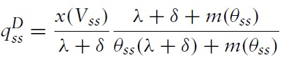
Since V_ss is falling in θ_ss from (uss), this implies that

is monotonically decreasing in θ_ss.

Next, setting U = U_ss,

implies a steady state supply function

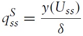
Since U_ss is rising in θ_ss from(uss), this implies that

is monotonically increasing in θ_ss. Thus, the demand and supply functions imply there exist a unique {q_ss, θ_ss} pair after setting

Comparative statics are intuitive. A greater flow of buyers in the form of higher x (for a given V_ss) implies higher q_ss, higher θ_ss and higher P_ss from (pss). A greater flow of production in the form of higher y (for a given U_ss) implies higher q_ss, lower θ_ss and lower P_ss. Lower π and higher r, δ, λ lead to lower q_ss. Higher z, β lead to lower θ_ss. While these comparative statics of steady state outcomes are interesting in their own right, a goal of this paper it to demonstrate the non-linear and gradual nature of transition paths that deviate from steady state outcomes.

The unemployment rate of the stock of goods is the share of goods held by sellers,

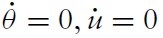
The dynamic equations (dynamics) imply the evolution of market tightness and unemployment rates are given by

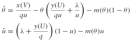
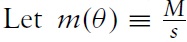
All derivations and proofs are in the Appendix. Let θ_θ (u,q,V,U), θ_u(u,q,U) denote the locus of solutions to

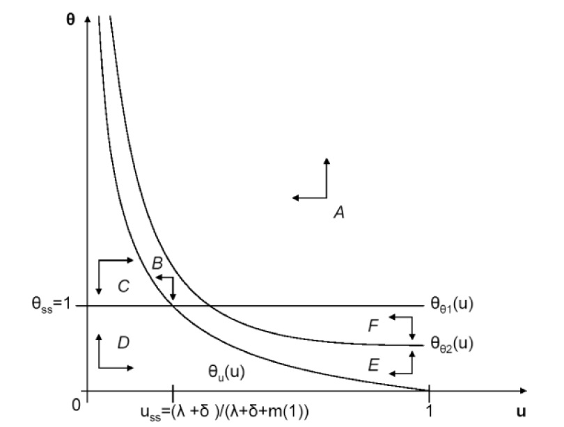
respectively. These equations will be applied to the analysis below of transition dynamics. The steady state tightness is given by

The steady state unemployment rate is u_ss = (λ + δ)/(m(θ_ss) + λ + δ).

The stock of goods never sold, or inventories, is distinct from the entire stock of goods. In the case where λ = 0, these are the same. The stock of inventories i, evolves according to

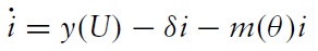
The evolution of inventories consists of the gross entry of new goods, minus gross exit through depreciation shocks and matches. The steady state level of inventories is given by i_ss = (y(U_ss))/(δ + m(θ_ss)).

The sales flow of the stock of inventories is m(θ)i, so the sales/inventory ratio is simply given by the liquidity of the good, m(θ). This implies that output y(U) and the sale/inventory ratio are positively correlated since U co-moves with θ from (asset).

We review three special cases to gain some analytical insight into the transition dynamics.Anecessary condition for a hangover effect is that prices and/or output deviate both above and below their steady state levels along a transition path following an innovation, which places these variables either above or below their steady state level. A goal of this section is to summarize as succinctly as possible the argument that necessary conditions for a hangover effect are:

(i) temporary exogenous innovations to the flow of buyers x, and

(ii) an elastic producer supply curve y(U).

This analysis then motivates a particular characterization of producer supply curves in the discussion of hangover effects discussed in Section 3.

Suppose demand and supply flows are perfectly inelastic such that the following holds.

Case 1.

is perfectly inelastic, and

is perfectly inelastic.

κ > 0 constant.

This implies that q is also constant. Under this assumption, equations (dynamics2) (see the Appendix) imply

Then the locus of solutions to

is given by

Note there are two solutions for θ_θ (u). Figure 2 plots the phase diagram in the {θ, u} space. There are six regions A − F bounded by the θ_θ (u), θ_u(u) loci.7 The steady state tightness is given by θ_ss = 1.

Temporary and exogenous innovations to x or y place the market in one of the six regions A − F. The associated transition paths are diverse. In particular, shocks that place the economy in region A, generate strong divergence in tightness θ and liquidity m(θ) from steady state levels before convergence. This divergence is associated with a positive feedback loop between liquidity and unemployment rates. Higher liquidity, lowers unemploymentwhich increases liquidity. Such overshooting effects are the focus of analysis in Kim (2009),where these paths a studied in more detail. Overall, innovations to x, y can have a large impact on priceswhen quantities are fixed.

However, none of the transition paths are associated with hangover effects in the following sense. If innovations to x, y place the market above (below) θ_ss, the market remains either above (below) θ_ss throughout the transition path. The associated prices U, which depend on the path of θ, are also always above (below) their steady state levels along the transition path.

In this special case, parameters were chosen such that one of the solutions for θ_θ (u) is θ_θ (u) = 1, which directly results in θ being always above (below) θ_ss = 1. While this is not necessarily the case for other settings with inelastic supply and demand, it is always the case that U (which depends on the path of θ) is above (below) U_ss along the transition path. 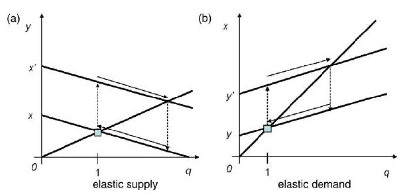Thus, hangover effects cannot be generated in settings of inelastic supply and inelastic demand.

Suppose supply flows are elastic, and demand flows are inelastic such that the following holds.

Case 2. y(U) is perfectly elastic at U = U(θ_ss = 1) > 0, and

is perfectly inelastic.

At an interior solution path where y > 0 always, we have θ = θ_ss = 1 always such that

and

The first equation is obtained from (dynamics2) after setting

Figure 3(a) plots these loci of points in the {y, q} space. It then plots the path of y following an exogenous temporary increase in

(a positive demand shock) from x to x’ which is anticipated. The initial steady state is indicated by the square point. The production of new goods y is above steady state levels, then below steady state levels along the transition path back to the steady state. This is a hangover effect in production. Note that this undershooting effect is a result of the fact that y is a decreasing function of q in the first equation of (yoyo).

Following a temporary decrease in

the reverse occurs.The flowof production y is below steady-state levels, then above steady-state levels along the transition path back to the steady state. Overall, innovations to x can have a large impact on quantitieswhen prices are fixed, and these dynamics are associated with hangover effects.8

Suppose supply flows are inelastic, and demand flows are elastic such that the following holds.9

Case 3.

is perfectly inelastic, and x(V) is perfectly elastic at V = V(θ_ss = 1) > 0.

At an interior solution path where x > 0 always, we have θ = θ_ss = 1 always such that

and

Again, the first equation is obtained from (dynamics2) after setting

Figure 3(b) plots these loci of points in the {x, q} space. It then plots the path of x following an exogenous temporary increase in

(a positive supply shock) from y to y’ which is anticipated. The initial steady state is indicated by the square point. The entry of new buyers x is always above the original steady state level along the transition path back to this steady state. Thus, there are no undershooting or overshooting effects present here.

Meanwhile, following a temporary decrease in

x is always below steady state levels along the transition path back to the steady state. Again, there are no undershooting or overshooting effects present.10 Thus, hangover effects cannot be generated in settings of inelastic supply and elastic demand.

7Region F exists iff the solutions   8It is possible that the transition path involves y = 0, its boundary value for a finite time interval, following both positive or negative demand shocks. At a non-interior solution path y = 0, U < U(θss = 1) such that   9This setting maps into the canonical search model of unemployment of Pissarides (2000). See the related discussion of rental markets in Section 6.  10Note that in this case, since x increasing in q in (w), we will never have a situation where x = 0, i.e. a non-interior point. Thus, in this case, we can rule out non-interior transition paths altogether.

The discussion above shows that hangover effects are generated through exogenous innovations in the entry rate of buyers x, when the producer supply function y(U) is elastic. In the rest of the analysis we keep the structure of buyer entry rates simple, inelastic and exogenous at

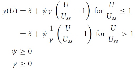
and focus on the implications of the elasticity of the supply function. This is conducted by considering a producer supply function that is (locally) characterized as

Setting γ = 1, ψ = 0 corresponds to the case of perfectly inelastic supply, and ψ =∞corresponds to the case of perfectly elastic supply. Under the formulation where γ < 1, there is a bias (kink) in the response of prices to output such that prices are inelastic upwards, but relatively elastic downwards.Conversely, if γ > 1, prices are elastic upwards, but relatively inelastic downwards.

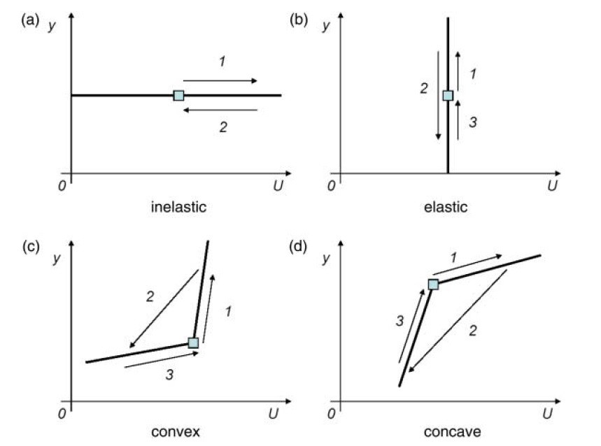
Figure 4 shows the effect of a temporary increase in the flow of buyers x on the price U and production y relative to their steady state levels, for a variety of specifications of y(U). In each case, the initial steady state is indicated by the square point. Panel 4(a) shows the case for inelastic supply (as discussed in Section 3). Prices rise and fall and output does not change. There are no hangover effects here. Panel 4(b) shows the case for elastic supply (as in Section 3). Only output changes and displays a hangover effect.

Panel 4(c) shows the case for a convex supply curve (i.e. γ < 1). The boom phase is characterized by a strong response of output relative to prices, and the hangover phase is characterized by a weak response of output relative to prices. Panel 4(d) shows the case for a concave supply curve (i.e. γ > 1). In this case, the boom phase is characterized by a weak response of output relative to prices, and the hangover phase is characterized by a strong response of output relative to prices.

The hangover effect plays out as follows.An exogenous and temporary increase in the entry rate of buyers initially causes liquidity m(θ), prices P and production y(U) to overshoot from the steady state levels due to a positive feedback loop between liquidity and the measure of sellers. This occurs because liquidity is increasing in the relative measure of buyers to sellers θ, and higher liquidity reduces the measure of sellers s, which increases liquidity. Meanwhile, a higher relative measure of buyers to sellers θ, raises prices P in favor of sellers, and induces higher production y(U). Thus, during this boom phase there is an expansion of the stock of goods q.

As liquidity peaks and then converges down to its steady state level, the stock of goods being sold s remains large relative to its steady state level. The necessary fall of production is signaled through a fall in liquidity and prices (a fall in the relative measure of buyers to sellers θ) to below steady state levels. This is the hangover phase. Finally, as the stock of goods q converges to its steady state level through lower production, and a gradual depreciation of goods at rate δ, liquidity, prices and production converge toward their steady state levels from below.

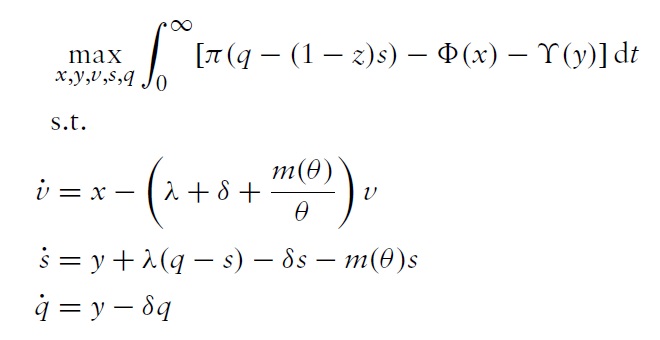
We can consider the optimization problem of a social planner who maximizes the discounted stream of earnings net of the costs of entry of buyers and producers, subject to the laws of motion for buyers, sellers and the stock of goods. The social planner problem is given by

where the initial v₀, s₀, q₀ are given. The market-wide buyer entry cost function satisfies Φ’(x) > 0, Φ”(x) ≥ and 0, and the production cost function satisfies ϒ’(y) > 0, ϒ”(y) ≥ 0. to map this problem into the decentralized market we also assume that the inverse function of Φ’(x) = V is the buyer entry function x(V), and the inverse function of ϒ(y) = U is the producer supply curve y(U).

Proposition 1 Under the Hosios (1990) condition β = η, decentralized outcomes coincide with outcomes chosen by the social planner.

By imposing the Hosios condition, we can interchangeably discuss decentralized outcomes and outcomes chosen by a social planner.

Arelated but different market structure that can be readily considered is the rental market for (durable) goods. In this case, buyers characterized above are potential renters with high earnings valuation π, and sellers are owners of goods with low earnings valuation πz. A match forms a bilateral union between renters and owners of goods for the duration of the match. π is the earnings from the good flowing exclusively to the renter during the match.When the match is terminated following a reassessment of earnings to πz by the renter at rate λ, the good reverts to the owner who searches for another renter, and derives a flow of earnings πz during the search. The match is also terminated upon the depreciation of the good at rate δ, in which case both renter and owner exit the market.

The rental rate w of the good is determined by a continuous process of Nash bargaining between these parties during the match, where β is the bargaining power of the owner. P now has the interpretation as the price of a good that is currently rented out, and U is the price of a good that is not currently rented out. The rental rate w is determined by

given

The flow value of a rented good rP, consists of the rental income flow w, plus the option value of a reassessment shock −λ(P − U), plus the option value of depreciation −δP, plus the capital gains

Given this reinterpretation, all other value equations remain the same as above in equations (asset).

Proposition 2 Outcomes for market tightness θ, and market prices P, are identical in rental markets.

Thus, whether goods are transacted through transfer of ownership or through rent is irrelevant for the market dynamics and price setting outcomes of goods.11 This allows us to discuss outcomes in both types of markets interchangeably.

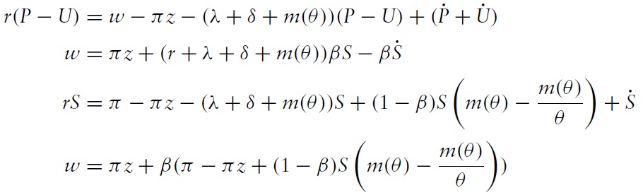
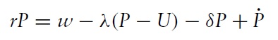
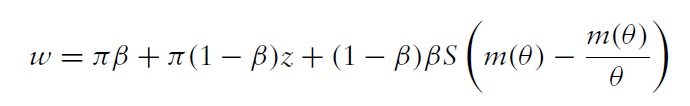
From (wage), (asset) and (nb), the rental rate can be expressed as:

This equation suggests that the rental rate w, can be inelastic relative to changes in tightness θ. In particular, the equation implies that when

wages are invariant to changes in θ. Such an argument may justify why large fluctuations in liquidity m(θ), and the associated fluctuations in unemployment rate u, and prices of goods P,U, are consistent with small fluctuations in their rental rates w, such as in the real estate market.

In the labor market, P,U translate into thewelfare of employed and unemployed workers respectively, which together with the unemployment rate u, can fluctuate widely despite inertia in the movement of wages w, the rental rate of labor. Such a wage stickiness prediction would not be delivered by a canonical search model of unemployment (Pissarides, 2000) for the following reason. In that framework, the value of buyers translates into the value of job vacancies, which are assumed to be fixed

The corresponding wage equation is given by:

which is increasing in θ. As mentioned already, this setting maps unto the market discussed in Section 4: inelastic supply and elastic demand.

11This corresponds to the insight in the canonical search unemployment model (Pissarides, 2000) that wages (a rental rate for labor) are irrelevant for determining market tightness.

This paper has shown that markets subject to frictions in the matching of buyers and sellers can generate hangover effects in the presence of adjustment costs to the entry of buyers and sellers. The analysis extends the insights of the canonical Ԛ-theory of investment to incorporate the correlation of liquidity with prices and production over cycles resulting from temporary, positive shocks. This generates dynamics for unemployment, inventories, sales and production consistent with documented patterns over the production cycle.

A direction for further study is the relationship between liquidity and the earnings of the good (which we took as constant). This is especially pertinent in the case of factor markets such as the labor market. In such markets, factor unemployment dynamics are associated with fluctuations in the earnings or productivity of the factor. Mortensen and Pissarides (1994) provide a canonical model of (labor) unemployment where liquidity affects the selection of matches such that average labor productivity is rising in liquidity. Combining the adjustment costs studied in the current paper with that framework could generate boom-bust cycles in labor productivity and unemployment as arising from temporary, positive shocks to the entry rate of new jobs (which rent labor services). If busts can really be viewed as the hangover of booms, we can improve our understanding of episodes of recessions, which seemingly occur despite an absence of large negative shocks.