Previous studies have shown that value premiums exist, not just in equity, but also in other asset classes. In the foreign exchange (FX) market, the profits of a strategy based on the deviation from purchasing power parity (PPP) as well as the profits of carry trades are considered value premiums.1 In the debt market, the profits of the yield curve slope-based strategy are interpreted as value premiums.2 In the commodities market, the strategy of buying commodities with a downward sloping forward curve, the so-called ‘backwardation-contango’ strategy, produces excess returns, which can be interpreted as value premiums.3 The investment strategies based on the ratios of current prices to past prices are also associated with value premiums.4
Given the multiplicity of value premiums inside and outside equity, the following questions naturally arise: What is the nature of the relationship among these value premiums? Are the value premiums in equity identical to the value premiums in other asset classes? Do they move together? Are they influenced by he same underlying factors?5
Two studies – those of Qian
The objective of the current study is twofold: (i) to present a possible explanation for discrepancy between two studies, those of Qian
To resolve the contradictory findings of the previous studies and to clarify the co-movement pattern of value premiums, we looked carefully at the correlation matrix of value premiums, conducted a principal component analysis, and also carried out a regression analysis. We also wanted to explore the practical implications of the co-movement pattern.We selected two applications to which the co-movement pattern is of particular relevance. These are value diversification and value timing. These applications illustrate the practical relevance of understanding the co-movement pattern.
We collected return series of 10 popular value-oriented investment strategies in four asset classes. Our list of value strategies is fairly comprehensive.We included the strategies addressed by Qian
Our analysis of the co-movement of returns reveals two distinct groups of value strategies. The returns of value strategies within a group move together, whereas the returns of value strategies belonging to different groups do not. Additionally, two groups have very different exposures to conventional equity risk factors. The existence of two distinct groups of value premiums and the components of these two groups explain the contradictory findings of the previous studies. The first group includes the yield strategy, the carry strategy, and the backwardation-contango strategy, in addition to all of the equity value strategies. The second group includes the PPP deviation strategy as well as the strategies selecting assets with low current prices relative to the prices of 5 years ago. This grouping corresponds to our intuition, as we explain below.
Many investors are of the view that buying a value stock is much like buying a high yield bond. The price-to-earnings ratio and the dividend yield of a stock are analogous to the current yield of a bond. All of them indicate how much gain investors anticipate from their investments. Investors expect to receive more from a low price-to-earnings or high dividend-yield stock, to the extent that current earnings or current dividends are indicative of future earnings or dividends. Similarly, investors expect to receive more from a high yield bond, to the extent that current yields are indicative of future payments. Buying a high yield bond is, in turn, similar to a carry trade. In a carry trade, one buys a high yield currency and sells a low yield currency in the hope that the decline in the value of the investment currency will not wipe out the interest differential between the investment currency and the funding currency. Buying a high yield asset produces above-average returns only if the price decline of this asset is not excessive. If the price of a high yield asset does not decline enough to eliminate all the profits, it is because of forward bias. If no forward bias exists, then the value of a high yield currency should equal the value of the forward rate, and there will be no profits deriving from the carry trade.6 A similar assertion can be made for value stocks and high yield bonds. That is, if no forward bias exists, buying a value stock or a high yield bond will not prove profitable. The backwardation-contango strategy is also based on forward bias. When the forward curve of a commodity slopes downward, this does not generally result in future price declines attributable to forward bias. Thus, buying such commodities generates excess returns.
Given the reasoning above, it is not surprising that the equity value strategies, the high yield strategy, the carry strategy, and the backwardation-contango strategy are all categorized into one group. It is also not surprising that all the other value strategies belong to another group. Selecting assets whose current prices are low relative to the past prices is similar to selecting long-term ‘losers.’ Thus, the profits of such selection strategies can be referred to as contrarian profits. The PPP deviation strategy is also used to identify long-term loser currencies, those currencies whose values have gone down. Thus, the profits of this strategy are also reflective of contrarian profits.
To illustrate the usefulness of identifying two groups among value premiums, we selected two applications: value diversification and value timing. To evaluate the benefit of value diversification, we calculated the mean-variance efficient frontiers out of different combinations of value premiums. We determined that the diversification benefit is significant when strategies are selected from both groups. The number of strategies included in the portfolio is not the most important aspect. Significant diversification benefit is achieved even with four strategies. For value timing, we focused on the timing of the price-to-earnings strategy. We employed two indicators – the number of positive value premiums and the average of value premiums. These indicators turned out to be useful in determining when to be long in the price-to-earnings strategy. To us, what is more noteworthy is that the effectiveness of the indicators is improved if we include value premiums from the first group only.
The remainder of the paper is organized as follows: in Section 2, we briefly comment on our construction of value strategies. A more complete description is presented in the Appendix. In Section 3, we analyze the co-movement pattern. In Sections 4 and 5, we discuss value diversification and value timing, respectively, and our conclusions are presented in Section 6.
1See Pojarliev and Levich (2008) and Qian et al. (2009). There is growing literature on carry trade and uncovered interest parity. See Brunnermeier et al. (2008) for an example of recent development. 2See Qian et al. (2009). 3The characterization of the backwardation-contango strategy as a value strategy is perhaps obvious, but has not been explicitly elucidated in the literature. This strategy is based on the idea of normal backwardation, which is originally attributed to Keynes (1930). Keynes assumed that speculators would take a long side. Carter (1983) relaxed this assumption and empirically examined ‘generalized normal backwardation’. Fort and Quirk (1988) provide more theoretical discussion. 4See Asness et al. (2009). Value premiums are often discussed in the context of style investing, e.g. Barberis and Shleifer (2003). The idea is that investors partition the investment universe into a small number of ‘styles’ and simplify their choice problem. Some authors take another view that there are different types of investors, i.e. they focus on the styles of investors. See, for example, Kim et al. (2008). 5Regarding the source of the value premium in the equity market, there are two lines of research, one focusing on the behavioral aspect and the other within the equilibrium framework. For the former, see De Bondt and Thaler (1985), Lakonishok et al. (1994), and Dechow and Sloan (1997). For the latter, see Fama and French (1995). 6See Engel (1996) for the discussion of the forward bias in the FX markets.
2. Value Premiums in Equity, Debt, FX, and Commodity
We examined value premiums in equity, debt, FX, and commodity. Table 1 lists the value premiums we examined for each asset class.
Different authors calculated value premiums in different ways. Qian
[Table 1.] Value premiums in equity, debt, FX, and commodity
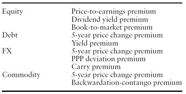
Value premiums in equity, debt, FX, and commodity

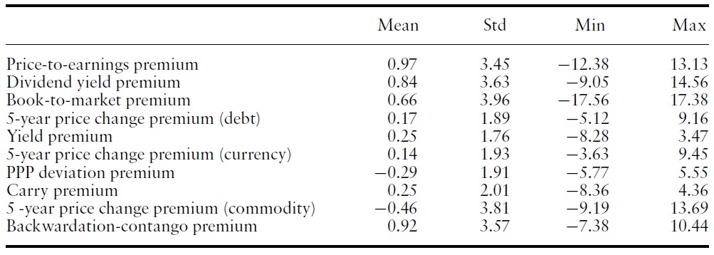
Univariate statistics of value premiums (all the value premiums can be interpreted as monthly returns on zero-investment portfolios. All the series are from January 1998 to December 2009)
Table 2 reports the univariate statistics of value premiums. They are based on monthly returns from 1998 to 2009.7 We were unable to extend our series further back into history, as government bond indices are not very reliable prior to 1993. Recall that we require 5 years of history for the calculations of value premiums. Additionally, global equity data are not very reliable before this time period.
7We conducted the analysis using weekly returns as well, and determined that the results were similar. In order to save space, we will discuss the results based on the monthly returns only.
3. Categorizing Value Premiums into Two Groups
In this section, we discuss the idea that two distinct groups of value premiums exist. We associate the first group with forward bias, and the second group with contrarian profits.
When asset A has a higher yield than asset B, it is rational to expect that the price of A will be lower than the price of B in the future. Thus, the forward price of A is lower than the forward price of B. This forward price, however, turns out not to be an accurate estimate of the future price. This is what we refer to as the forward bias. Many of the value premiums we described in the previous section can be associated with forward bias. The yield premium, the carry premium, and the backwardation-contango premium are all related directly to the forward bias. The yield premium and the carry premium are based on the yield differential, which can be translated into the forward price differential. The backwardation-contango premium is predicated on the forward price differential. The price-to-earnings premium and the dividend yield premium can be similarly understood. The price-to-earnings ratio is the inverse of the earnings yield. We argue below that the book-to-market premium is quite similar to the other value premiums associated with forward bias.Thus,we also include the book-to-market premium in the first group.
Buying ‘losers’ and selling ‘winners’ is referred to as the contrarian strategy. Certain value strategies can be regarded as contrarian strategies. Comparing current prices to past prices and buying those assets whose current prices are low relative to past prices is a contrarian strategy. The 5-year price change premiums we described in the previous section fall into this category. The PPP deviation premium belongs to this category as well, in the sense that the PPP primarily reflects past exchange rates.
The remainder of this section has three parts: in the first part, we motivate the idea of dividing value premiums into two groups from our analysis of the correlation matrix. In the second part, we examine the principal components and interpret the first two principal components as representing the co-movements of two groups. In the final part, we assess the relationship of value premiums to conventional equity risk factors, and assert that the two groups of value premiums are distinctly related to equity risk factors.
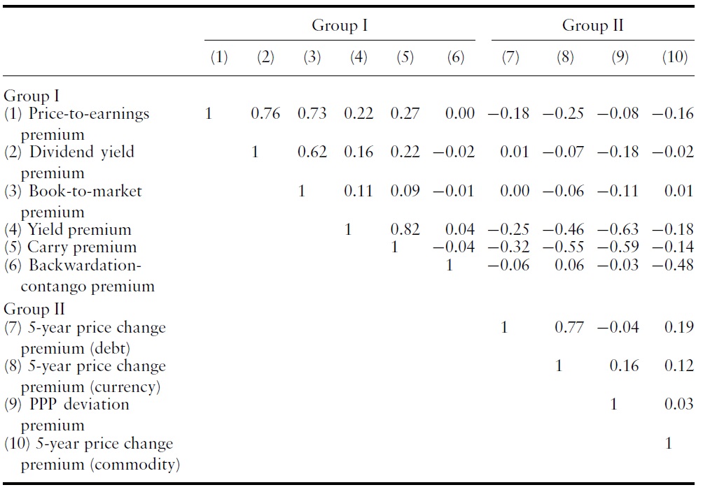
In Table 3, we grouped together those value premiums that were correlated positively with the price-to-earnings premiums (Group I), and subsequently grouped together the remaining premiums (Group II). The validity of this grouping can be confirmed by the following three observations: (1) Elements in the upper left block are largely positive, thereby indicating that the value premiums in Group I are similar to one another. (2) Elements in the lower right block are mostly positive, thus indicating that the value premiums in Group II are also similar to one another. (3) Elements in the upper right block are largely negative, thus indicating that Group I and Group II are quite negatively correlated.

Correlation matrix of value premiums (monthly value premiums from January 1998 to December 2009 are used for this calculation)
Eigenvalues and eigenvectors of covariance matrix (monthly value premiums from January 1998 to December 2009 are used for this calculation)
We associate the value premiums in Group I with forward bias and those in Group II with contrarian profits, as discussed previously.While this distinction is not based on a comprehensive theory of all the value premiums, we argue below that this distinction makes sense, and that the distinction is useful.
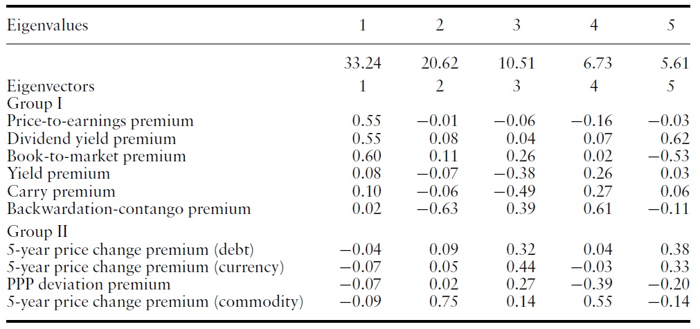
To construct principal components out of the value premiums, we calculated the eigenvalues and eigenvectors of the covariance matrix. As there are 10 value premiums, there are 10 eigenvalues and 10 eigenvectors after conventional normalization. Table 4 shows the largest five eigenvalues and the associated eigenvectors.
The first eigenvector has positive elements for value premiums in Group I and negative elements for value premiums in Group II. Therefore, it is natural to interpret the first principal component as being reflective of the return differential between value premiums in Groups I and II. Looking at the eigenvalues, the first principal component represents approximately 40% of the total eigenvalues. Thus, the distinction between value premiums in Group I and Group II is the single most significant pattern of the covariance matrix.
The second eigenvector exhibits positive values for the dividend yield premium and the book-to-market premium, as well as for value premiums in Group II. That is, the second eigenvector has precisely opposite signs from the first eigenvector, with the exception of the dividend yield premium and the bookto-market premium. Thus, we interpret the second principal component as representing the returns of the dividend yield premium and the book-to-market premium in excess of the first principal component. Similarly, the third principal component represents the unique return of the backwardation-contango premium.
3.3 Relation to Conventional Equity Risk Factors
We attempted to determine the manner in which each value premium is related to conventional equity risk factors.We recognized that equity risk models are for equity, and not for other asset classes.However, considering the lack of a standard risk model for non-equity assets, we felt justified in looking at the relationship between various value premiums and equity risk factors. Additionally, equity risk factors may capture some of the risks of non-equity assets.
We employed a five-factor model in which we included the market factor, the size factor, the price-to-earnings factor, the momentum factor, and the leverage factor. Compared with the conventional Fama-French model, the additional factors we included were the momentum factor and the leverage factor. For the price-to-earnings factor we used the actual earnings of the past fiscal year. Otherwise, this factor was calculated in the same way as the price-to-earnings premium described in the previous sections.8,9 The size factor, the momentum factor, and the leverage factor were also calculated similarly. The size factor is the difference between the returns of the small stock portfolio and the large stock portfolio. The small stock portfolio includes those stocks residing within the bottom 50%, and the large stock portfolio includes those stocks in the top 10%.10 The momentum factor is the difference between the returns of the high momentum portfolio and the low momentum portfolio. The high momentum portfolio includes those stocks in the bottom 25% of the 6-month momentum ranking, and the low momentum portfolio includes those stocks in the top 25%. The leverage factor is the difference between the returns of the high leverage portfolio and those of the low leverage portfolio. The high leverage portfolio includes those stocks in the top 25% of the ranking by leverage, and the low leverage portfolio includes those stocks ranked in the bottom 25%. Leverage is defined as the total liabilities over equity.
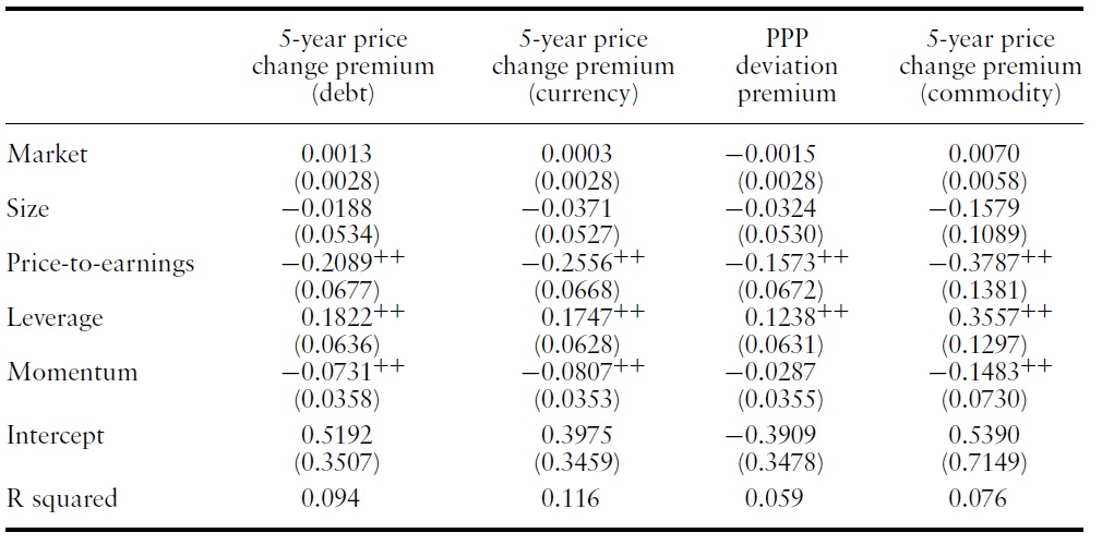
Tables 5 and 6 show the estimates of the five-factor model for each value premium.11 For the value premiums in Group I, the price-to-earnings factor is consistently significantly positive. The leverage factor is significantly negative for all but the book-to-market premium. Contrary to this pattern, for the value premiums in Group II, the price-to-earnings factor is consistently significantly negative and the leverage factor is always significantly positive.
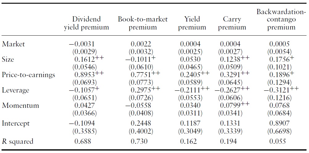
Explaining value premiums (Group I) by equity risk factors (monthly value premiums from January 1998 to December 2009 are used for this calculation. ++indicates significance at 5% and +indicates significance at 10%)

Explaining value premiums (Group II) by equity risk factors (monthly value premiums from January 1998 to December 2009 are used for this calculation. ++indicates significance at 5% and +indicates significance at 10%)
For the yield and carry premiums, the size, the momentum, and the priceto-earnings factors are significantly positive, whereas the leverage factor is significantly negative. A similar pattern is observed for the backwardationcontango premium, although the size factor is not significant and other risk factors are only marginally significant. For the last three premiums, the opposite pattern is observed. The size, the momentum, and the price-to-earnings factors are negative,whereas the leverage factor is positive. Momentum is largely negative for value premiums in Group II.

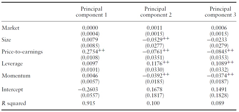
Explaining principal components by equity risk factors (monthly value premiums from January 1998 to December 2009 are used for this calculation. ++indicates significance at 5% and +indicates significance at 10%)
These results support our categorization of value premiums into Group I and Group II. Value premiums have similar coefficients within each group and very different coefficients across groups. Value premiums in Group I co-vary positively with the price-to-earnings factor. Value premiums in Group II co-vary positively with the leverage factor.
Table 7 shows the relation of principal components to equity risk factors. Unsurprisingly, principal component 1 exhibits a pattern similar to that of the value premiums in Group I, whereas principal components 2 and 3 exhibit a pattern similar to that of the value premiums in Group II.
As mentioned earlier, the significance of the results reported in Table 6 and 7 depends on the ability of equity risk factors to price non-equity assets. The analysis would improve if there are proper asset pricing models relevant for multi-asset classes.12
8It makes no difference whether we employ actual earnings or forward earnings. We used actual earnings here, as these appear to be more popular as a risk factor. 9We used the price-to-earnings factor rather than the book-to-market factor used in Fama–French model, simply because price-to-earnings are easier to interpret for our purposes. Price-to-earnings are more closely related to the notion of forward bias, whereas the book-to-market can be interpreted variously. If current earnings are good indicators of future earnings, price-to-earnings can be interested as a measure of ‘how much investors are willing to pay for one dollar of future earnings.’ To put it another way, low price-to-earnings stocks are high-yield stocks; when high-yield stocks have high returns, we may relate it to forward bias. It is more difficult to related book-to-market to forward bias; book-to-market is not directly related to the idea of yield. 10We do not use 25% as the cutoff level for the size portfolios as the resulting portfolios would be quite different from what is conventionally considered small-cap stocks and large-cap stocks. To put it another way, the number of small cap stocks is much greater than the number of large cap stocks, which requires a higher cutoff level for the small-cap portfolio and a lower cutoff level for a large-cap portfolio. 11We did not include the price-to-earnings premium, because it is very similar to the price-toearnings factor. 12A more thorough examination of the relationship between various value premiums and equity P/E and leverage factors is left as a future research agenda.
We examined two applications to show the advantage of categorizing value premiums into Group I and Group II. In this section,we discuss value diversification, and in the following section we discuss value timing.
While many believe that ‘value investing’ will reward investors in the long run, maintaining constant exposure to a particular value premium entails a significant level of risk. For these value investors, whether or not one can reduce risk while being exposed constantly to value is an important question.
After addressing this question, Qian
Our analysis explains why these two studies drew opposing conclusions. Put simply, value premiums within Group I and also within Group II are highly correlated, and the diversification benefit is limited if one invests only in the value premiums of Group I or only in the value premiums of Group II. However, if one invests both in the value premiums of Group I and Group II, then much more diversification benefit can be generated.
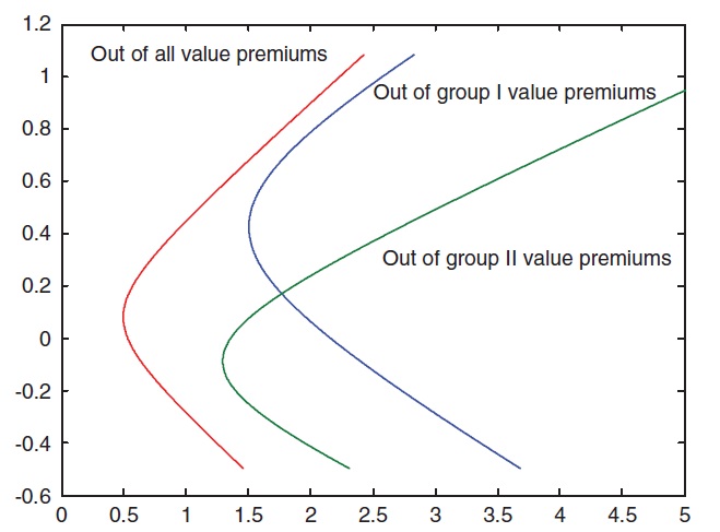
To illustrate this notion, Figure 1 plots the efficient frontiers out of the value premiums in Group I, out of the value premiums in Group II, and out of all the value premiums.Table 8 reports the related statistics.The investment opportunity is significantly expanded as we combine the Group I value premiums and Group II value premiums. The maximum Sharpe ratio of the efficient frontiers out of the Group I value premiums is 0.394, whereas the maximum Sharpe ratio of the efficient frontiers out of all value premiums is 0.452. These numbers are based on annualized returns.
It is natural that the investment opportunity set expands as the number of assets increases. Thus, there is nothing surprising in that the maximum Sharpe ratio increases when Group I and Group II are combined.What we really liked to show is that the maximum Sharpe ratio increases significantly if we select value premiums from Group I and Group II,
The second panel of Table 8 showsthemaximumSharpe ratio and the minimum standard deviation when we select each additional value premium to maximize the maximum Sharpe ratio. That is, if we are to select only one value premium, then we may choose the price-to-earnings premium, because it has the largest Sharpe ratio. If we are to add one more value premium to the price-to-earnings premium, then we would select the backwardation-contango premium, as this would maximize the maximum Sharpe ratio. Given the ability to add one more, our next choice would be the 5-year price change premium (debt).
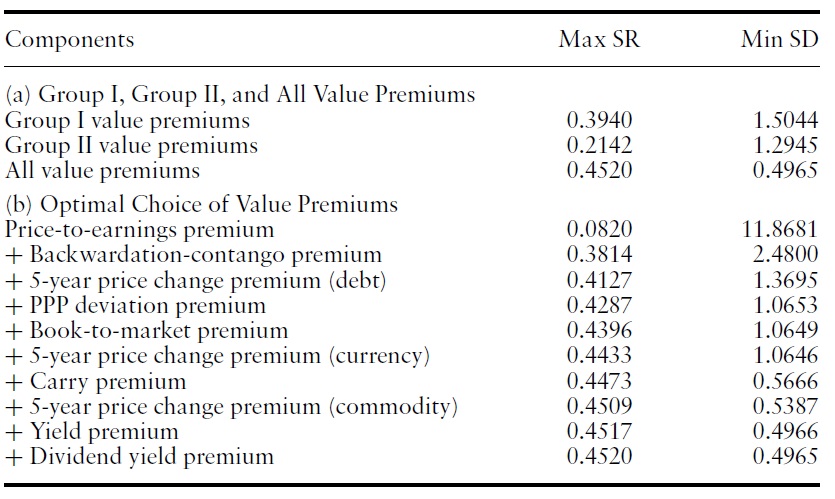
Maximum Sharpe ratios and minimum standard deviations (Sharpe ratio and standard deviation are based on annualized returns. For the calculation of Sharpe ratio, the risk-free rate of 0% is assumed. Value premiums from January 1998 to December 2009 are used for this calculation)
We make two observations regarding panel (b). First, the optimal combination of value premiums in terms of the maximum Sharpe ratio is achieved when we combine the Group I value premiums with the Group II value premiums. The first two premiums are from Group I, while the next two premiums are from Group II. The fifth choice is from Group I, and the sixth choice is from Group II. The second observation is that not much gain occurs once we have more than three value premiums. The greatest diversification benefit is achieved if we select two value premiums from Group I and one or two value premiums from Group II.
That the first two premiums are from Group I suggests that if one is restricted to choose only two, only Group I premiums will be selected and there will be no mixing of Group I and Group II. Note, however, that ifwe look at all possible twopremium combinations, mixing of Group I and Group II is more often superior to mixing within Group I or Group II. For example, mixing price-to-earnings premium with one of 5-year price change premium (debt), 5-year price change premium (currency), and 5-year price change premium (commodity), and PPP deviation premium is superior to mixing price-to-earnings premium with one of book-to-market premium, carry premium, yield premium, and divided yield premium.
The marginal gains in the maximum Sharpe ratio and the minimum standard deviation are greater when two premiums are selected than when three or more premiums are selected. This pattern is not surprising. It is natural to have large marginal gains initially.With the combination of price-to-earnings premium and backwardation-contango premium, the maximum Sharpe ratio is 0.38.We obtain smaller, but comparable maximum Sharpe ratios from other two-premium combinations. For example, when we mix price-to-earnings premium with one of one of 5-year price change premium (debt), 5-year price change premium (currency), and 5-year price change premium (commodity), and PPP deviation premium, the maximum Sharpe ratio is between 0.31 and 0.32.
To enhance the performance of a value strategy, one may consider value timing, i.e. switching in and out of value depending on the market conditions. A few alternatives for carrying out value timing in equity markets have been introduced in the relevant literature.13 Kao and Shumaker (1999) employed macroeconomic variables as predictors of value performance, whereas Asness
Given the co-movement pattern of value premiumswe discussed in the previous sections, we evaluated the possibility of using the aggregate of multiple value premiums as a predictor of the future value of the price-to-earnings premium. To the extent that different value premiums reflect some common underlying factors, joint upward movement of different value premiums may indicate the strength of the underlying factors. When a larger number of value premiums are positive, the value effect may be stronger and may last longer. Thus, we considered the number of value premiums that are currently positive, as well as the average of value premiums.
We recognize the difficulty of devising a successful value timing strategy and the limitation of evaluating a strategy with relatively short time-series data. Thus, our principal objective in this section is in illustrating the benefit inherent to categorizing value premiums into two groups.We argue below that the efficacy of value timing is not significantly enhanced by considering value premiums in the other group. That is, in predicting the price-to-earnings premium, it is effective enough to consider value premiums that belong to the same group, i.e. Group I.
Our analysis proceeded as follows: at the end of January 1998, we counted the number of positive value premiums in Group I. We normalized this number by dividing by the total count. The resultant indicator is always between 0 and 1. If this indicator was greater than the critical value
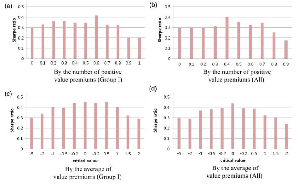
When the critical value for the number of positive value premiums is 0, we always take a long position in the price-to-earnings strategy. Thus, there is no value timing. In this case, the Sharpe ratio is approximately 0.3. As the critical value becomes larger, however, the Sharpe ratio increases. In plot (a), wherein the Group II value premiums are not considered, the Sharpe ratio peaks at 0.4 when the critical value is 0.6. In plot (b), wherein the Group II value premiums are also considered, the Sharpe ratio peaks at 0.4 again, but this time when the critical value is 0.4. Overall, we see no significant improvement from plot (a) to plot (b).
When value timing is based on the average of value premiums, a similar pattern arises. Including the Group II value premiums in the calculation of average results in no significant improvements. In fact, the opposite appears to be the case. The Sharpe ratio is somewhat higher when Group II value premiums are not included, which can be seen in panels (c) and (d).
Therefore, our conclusion is as follows: while the aggregate of value premiums has potential use in value timing, in calculating the aggregate, we do not need to consider value premiums in the other group. In this regard, our categorization of value premiums is of practical relevance.
13While we focus herein on the equity value timing, the timing of the FX value, especially carry, is also discussed in the literature. See Brière and Drut (2009), and Melvyn and Taylor (2009). 14Gulen et al. (2010) used the Markov-switching model to study time-variation in the expected value premium. With regard to the predictability of value premiums, their conclusion was in the negative. 15Assuming 0% interest for cash is a conservative choice for our analysis.
Two goals of this paper was to present a possible explanation for discrepancy between two studies, those of Qian
To illustrate the usefulness of categorizing value premiums into two groups,we considered two applications in which such categorization appears relevant. First, if investors pursue diversification among value strategies, it is important to include value strategies from both groups. This is particularly relevant when transaction costs limit the number of strategies to be included in the overall portfolio. Second, if investors pursue value timing based on some indicators predicated on multiple value premiums, there is little gain to be had in basing the indicator on all the value premiums. It is sufficient, and sometimes even better, to consider only the value premiums that belong to the same group as the investment vehicle.