Due to the latest economic downturn, the public (and academic) debate about monetary policy in the Euro area has flared up again. Although under some political pressure, the European Central Bank (ECB) adheres to its principle of stabilizing the price level. Compared to its US counterpart, the Federal Reserve System (Fed), the ECB uses monetary policy in order to stabilize the economy, but it does so very tentatively. This policy is in line with some of the cutting-edge models used for advice regarding monetary policy. Strict price-level targeting corresponds to the recent emphasis in modeling economies within theNewKeynesian (NK) framework on stabilizing the output gap. In this setting, there is no trade-off between price stability and the stability of output around potential. In the last few years, this modeling framework has become very popular as a theoretical basis for policy decisions forWestern central banks. This dynamic modeling approach assumes imperfect competition in the goods market and sluggish nominal price adjustment. Inspired by a seminal paper of Clarida
The formation of a monetary union in Europe and the debate about the ‘Stability and Growth Pact’ (SGP) make the analysis of fiscal and monetary interactions an especially important topic. It is often argued that the loss of monetary policy flexibility due to the merger of currencies increases the potential role of fiscal policy as a stabilization tool and the need for cooperation within Europe with regard to fiscal policy. Therefore, to optimally characterize policy in the European Monetary Union (EMU), the fiscal stance has to be taken into account. The interaction of monetary and fiscal policy in a NK modeling framework has been examined, for instance, by Corsetti and Pesenti (2001) and Schmitt-Grohé and Uribe (2004) (for a closed economy) or by Lombardo and Sutherland (2004) and Leith and Wren-Lewis (2008) (for an open economy).
Despite its potential relevance for political decision makers, only a few papers considering monetary and fiscal aspects in a currency union have been written in recent years. Most of the existing literature that does analyzes monetary and fiscal policy within a micro-founded, two-country sticky-price model of a monetary union (e.g. Beetsma and Jensen, 2005; Ferrero, 2009). As a two-country approach may be useful for discussing issues concerning the interaction between two large economies (e.g. the EU and the US), it can hardly be viewed as a realistic description of a monetary union such as the EMU, which currently has 16 member states. Just recently, Galí and Monacelli (2008) proposed a framework that incorporates the features mentioned above but comprises many open economies linked by trade and financial flows. As most of the member states of the EMU are small relative to the union as a whole, domestic policy decisions have little impact on other member states. Next to a more realistic modeling approach, this framework provides the possibility of studying policy problems for a single member country considered in isolation. The implications for monetary and fiscal policy, however, are (qualitatively) similar: (a) the common central bank never faces a trade-off between stabilizing output and inflation (i.e., stabilizing the price level is always optimal), and (b) an active domestic fiscal policy is only justified by the inefficient response of the terms of trade.
After having been largely ignored by monetary economists for a long time, the importance of real rigidities for monetary policy has received fresh impetus with a recent paper by Blanchard and Galí (2007). They show that including rigid real wages in a NK business-cycle model leads to a notable trade-off between stabilizing the price level and the welfare-relevant output gap. Moreover, as already highlighted in Galí
Real wage rigidity indeed seems to be an important feature of European labor markets. As found by Apaia and Pichelmann (2007), who use micro data from all EMU countries, the half-lives of deviations of the real wages from their equilibrium level vary between three quarters and three years.
As a result, in the analysis of European-wide monetary and fiscal policy design, realwage rigidity can hardly be neglected. Despite its importance, research in this direction its still in its infancy. Campolmi and Faia (2006) and Abbritti (2007) are the first (and as far as I knowremain the only) authors to include realwage rigidity in a dynamic model of a currency union.
Thus, in my opinion, an analytical framework of the EMU should have the following four properties: it has to rely on the assumptions of standard NK theory (i.e. imperfect competition and nominal rigidities), should include a monetary and fiscal authority, has to comprise many open economies (not only two), and has to incorporate real rigidities.
The model I propose in this paper meets all desiderata listed above. More precisely, I use a version of the Galí and Monacelli (2008) model extended by a partial adjustment process of the real wage and households as monopolistic labor suppliers. I focus on policy rules that are optimal (in welfare terms) from the union’s and not from the national perspective. This implies that union-wide monetary policy and domestic fiscal policy are perfectly coordinated to maximize overall welfare. Moreover, I assume that both fiscal and monetary authorities implement Ramsey solutions (i.e., optimal commitment strategies).
The main findings of the analysis are as follows. Because I assume that a single member country has no impact on union-wide economic conditions, an idiosyncratic shock does not affect union-wide economic dynamics. Therefore, the common central bank has no need to intervene. However, if each member country is affected by a shock (or it is not idiosyncratic), the common central bank faces a trade-off between stabilizing the price level and the welfare-relevant output. The quantitative simulations show that the optimal volatility of inflation (relative to output gap volatility) increases with the importance of real rigidities. This stands in contrast with the findings of Galí and Monacelli (2008). Furthermore, I find that optimal domestic fiscal policy also plays a national stabilization role if shocks are symmetric, as rigid realwages are an additional source of a tradeoff, along with inefficient adjustments in terms of trade. The basic rationale for this is simple. Rigid real wages prevent marginal costs from adjusting efficiently. This causes pressure on the national price level. To dampen (dis)inflation, the optimal policy absorbs the (dis)inflationary pressure by a change in output (relative to its efficient outcome), which has to be stimulated to some degree by national fiscal policy. Because optimal domestic fiscal policy has an important stabilizing role, from a union-wide perspective, external constraints such as the SGP should be seen in a different light.
The remainder of this paper is set out as follows: section 2 describes the related literature. The underlying model is outlined in section 3. Then, a short overview of the implementation method is given, and the baseline calibration of the model is presented. The results of the analysis are reported in section 6. Section 7 concludes.
An extensive amount of work has been done on monetary policy in micro-founded models with sticky prices. Additionally, the interaction between monetary and fiscal policy in such a framework has been analyzed in recent years (e.g., Schmidt-Grohe & Uribe, 2004, or Leith & Wren-Lewis, 2008). Although it has become acutely important with the creation of the EMU, multi-country versions of these models have attained less attention. Benigno (2004) analyzes the optimal monetary policy in a two-country framework. Neglecting the role of fiscal policy, he shows that in the presence of idiosyncratic shocks to technology, stabilizing the price level is desirable from a welfare perspective. In a similar setting but including national fiscal authorities, Beetsma and Jensen (2005) furthermore find evidence that countercyclical spending on national level iswelfare enhancing from a union-wide perspective. As aforementioned, Galí and Monacelli (2008) also study optimal monetary policy and the role of fiscal stabilization. However, in a multi-country framework, they derive quite similar implications for how monetary and fiscal policy should be implemented. Based on the Galí and Monacelli (2007) model, Forlati (2007) analyzes fiscal policy under no-coordination. She finds that the normative prescriptions emphasized by the authors mentioned above are no longer valid once policymakers are not coordinated. In this case, optimal monetary policy does not imply that the central bank stabilizes the average union inflation, as it has to take into account the distortions caused by the lack of coordination among fiscal policymakers. Ferrero (2009) additionally examines the role of distortionary taxation in a two-country framework, again from a union-wide perspective. In his setting, monetary policy should achieve aggregate price level stability, while fiscal policy should stabilize country-specific shocks via permanent variations of government spending and tax gaps but abstain from creating inflationary expectations at the union level.
A first step in introducing real rigidities in a two-country model of a currency union is taken by Campolmi and Faia (2006). They focus on the investigation of the impact of labor-market imperfections on inflation differentials between members rather than on optimal policies. Closer to the framework used in this paper is the modeling approach used in Abbritti (2007). However, Abbritti considers a world consisting of only two countries and additionally assumes market rigidities, which generate involuntary unemployment. He introduces a real wage rigidity that follows a stochastic process. Furthermore, the studies of Campolmi and Faia (2006) and Abbritti (2007) do not include a fiscal sector in their analysis; neither is a welfare analysis or a derivation of optimal policies part of their analysis.
In addition to the literature on sticky price models of a currency union, papers using real wage rigidities in NK models should be briefly reviewed. Just recently Blanchard and Galí (2007) reconsider the impact of rigid real wages on monetary policy design in a closed economy. Within a basic NK model, they show that the presence of the inertial adjustment of real wages leads to a notable tradeoff in monetary policy design. They find that under this additional assumption, there is a trade-off between stabilizing inflation and the welfare-relevant output. Moreover, they find that taking into account rigid real wages is a crucial element in understanding persistent inflation.
Next to sticky inflation dynamics, real wage rigidity can also help to explain observed labor-market fluctuations. As shown by Hall (2005) and Shimer (2005) real wage rigidity is necessary to explain the large cyclical variation in job vacancies.1
In spired by these papers, some richer sticky price models with rigid real wages – additionally considering labor-market frictions – have been developed (e.g. Christoffel & Linzert, 2005; Faia, 2008).
Especially in European countries, inertial adjustment in real wages seems to be an important feature for properly understanding labor market dynamics. It is often argued that European labor markets are rigid in many perspectives. High firing costs and unemployment benefits and collectivewage bargaining in particular prevent wages fromadjusting instantaneously. There is a lot of micro-founded theory for possible reasons intensifying this rigidity. Among others, one could mention efficient wage contracts, loss aversion, strong union power, or fairness considerations.2 Empirical evidence for rigid real wages has been given by a number of studies in recent years.3 They all attest relatively high real wage rigidity in the EU (compared with the US).
1However, the effects of real wage rigidity are still matter of some controversy. See, for instance, Mortensen and Nagypál (2007) for a critical review. 2For instance, Bewley (1999) provides an overview of recent research in this direction. 3See, for example, Bauer et al. (2007), Barwell and Schweitzer (2007), Deviciente et al. (2007), Dickens et al. (2007), Du Caju et al. (2007), Heckel et al. (2008), Holden and Wulfsberg (2007).
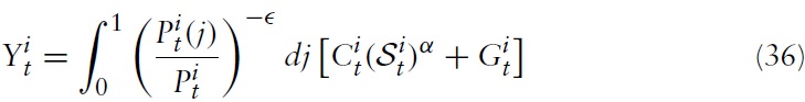
The model I use to derive the optimal monetary and fiscal policy in a currency union is, in the spirit of Galí and Monacelli (2008), a variant of a dynamic New Keynesian (NK) model applied to a mass of small open economies sharing the same currency. The world consists of a continuum of small open economies indexed by
Consider a typical country belonging to the union, say, country
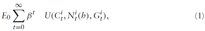
where

with χ ∈ (0, 1) as a weight attached to public consumption. That is, preferences are defined over the consumption of private and public goods,
and labor

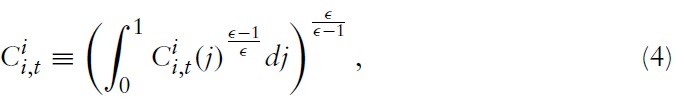
which is assumed to be immobile across countries.4 The composite of private consumption is defined by
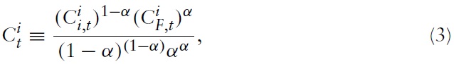
where

represents the household’s consumption of domestic goods. Formally,

is a CES aggregation of all goods produced in country

where
Nevertheless, people in country

The home bias in private consumption is denoted as 1 − α. Alternatively, α can be understood as an ‘index of openness’ in country
The representative household in country

for all
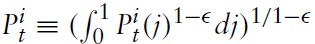
represents an index of prices of all domestically produced goods, for all
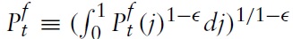
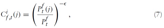
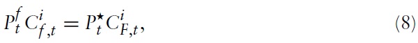
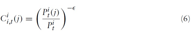
as a (producer) price index for the bundle of goods imported fromcountry f . It follows from equations (6) and (7) that


Moreover, the optimal allocation of expenditures implies

for all
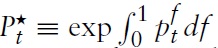
denotes the union-wide price index. Note that from the perspective of any individual country,

is also the price index of imported goods.
Next, one can define the consumer price index (CPI) as
It follows that one can write the optimal allocation of expenditures between domestic and imported goods, respectively, in country


At this point, one can combine the previous results to write the total (optimal) consumption expenditures of the representative household in country

As usual, maximization of equation (1) is subject to a sequence of flow budget constraints given by

where Wt(

represents the quantity of oneperiod, nominal risk less discount bonds purchased in period

is a lump-sum component of income, which may include, among other items, lump-sum taxes, dividends from the ownership of (domestic) firms, etc.
Given optimal allocation of expenditures, the household’s period budget constraint can be written as

Additionally, the household is assumed to be a monopolistic competitive supplier of labor facing the following constant-elasticity labor demand function


is country

its aggregate nominalwage index defined as
Maximizing equation (1) with respect to
and subject to equations (13), (14) and a solvency constraint, leads to the optimality conditions:
where
is the optimal wage markup in country

= 1/(Et{Ԛt,t+1}) denotes the usual gross nominal one-period return. Alternatively, one can write the marginal rate of substitution (MRS) between consumption and leisure in equation (16) and the Euler equation in equation (17) in log-linearized form (henceforth, lower-case letters denote the logs of the respective variables):


where the CPI inflation is defined as

and
Note that because no worker is unable to set a nominal wage at any time (e.g. through a staggered wage-setting scheme as in Erceg
in the remainder. Otherwise, I allow for exogenous variations in the markup due to shifts in

which can be interpreted as the exogenous variation in workers’ market power or, more generally (as it is modeled here), as a cost-push shock on the firm side.5 It is assumed that

is equal to a normally distributed, serially uncorrelated innovation with zero mean and finite variance

3.1.1 Some definitions and identities
Before proceeding with the analysis, I introduce some definitions and identities that I will need in what follows. First, I define the effective terms of trade between two countries, say, country
Consequently, I define the effective terms of trade for country
Alternatively, writing equation (21) in logs yields
Using the definition of CPI and equation (21), one can relate

and the domestic price level

according to

or in logs:

Subtracting a lagged version of equation (23) from the same equation, one can also relate domestic inflation, i.e.,

and CPI inflation according to

This makes it clear that the gap between CPI inflation and domestic inflation is equal to the percentage (as it is expressed in logs) change in terms of trade relative to the index of openness.Obviously, considering the aggregate price level, one has

and hence

as the terms of trade clearly vanish for the union as awhole. Formally, this can be seen by integrating equation (23) over
Furthermore, it is assumed that financial markets are complete at both the domestic and the international level. This assumption implies perfect consumption risk sharing within each country and the equalization of the marginal utilities of consumption between countries. Using the definition for the bilateral terms of trade, the risk-sharing condition can be expressed as

for all


where

3.1.2 Introducing real wage rigidities
In Europe (and to some degree in the US), there are no sudden and significant shifts in the aggregatewage level observed. Moreover, due to collectivewage-bargaining agreements, wages change only infrequently. As a result, a wage that can be freely adjusted in each period is hardly consistent with (European) reality. For this reason, many authors have recently focused on the examination of sluggish wage adjustment.
Erceg
Hall (2005) proposes a modeling strategy of sluggish wage adjustment that improves the cyclical properties of labor-market models. He introduces wage rigidity as a constant wage rule, which may be interpreted as a wage norm or social consensus. In this paper, we use a version of Hall’s notion of a wage norm in order to introduce real wage rigidity. In particular, it is assumed that the real wage

paid to a worker in country

and a wage norm

that is,

with 0 ≤

and

I thus assume a partial adjustment model of the form

or written in logs

where
The monetary-policy instrument of the common monetary authority is the union-wide nominal interest rate

Following Woodford (2003), the model abstracts from monetary frictions and considers the limit of a ‘cashless economy’. Seigniorage thus does not represent a source of revenues for national governments.
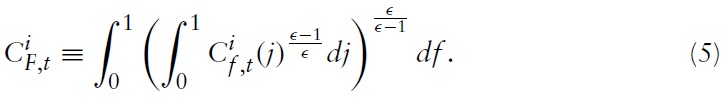
In contrast to the nominal interest rate, the government purchases are not common across all member countries. As with the private consumption of domestic and imported goods, I define country

as a CES aggregation of all public consumption goods available:
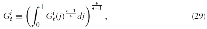
where

denotes the consumption of good
To simplify matters, I assume that public spending is financed by lump-sum taxation, so that Ricardian equivalence holds.
In any individual country, a continuum of firms produces a single good each, indexed by

where

is a country-specific exogenous stochastic technological factor common to all firms in the respective country. This productivity shifter is assumed to follow an AR(1) process, given by:

with
The labor used by each firm
Aggregating over all profit-maximizing firms in the domestic economy finally yields the labor demand in equation (14). Because in equilibrium each household in country

Due to the labor subsidy, the firms’ profits per unit of productivity are
for all

Additionally, firms are subject to some constraints on the frequency withwhich they can adjust their prices of the goods they sell.Acurrent modeling strategy is to use the formalism proposed in Calvo (1983). That is, each firm may reset its price only with probability 1 −

where

denotes the log of newly set prices in country
In this section, I summarize conditions determining the dynamic equilibrium of the system. The following definition characterizes an equilibrium for every member country of the currency union:
Definition 1

I show in the following that an equilibrium according to this definition can be summarized – for the national level and for the union as a whole, respectively – by just two equations: the domestic (resp. union-wide) dynamic IS equation, and the domestic (resp. union-wide) ‘New-Keynesian Phillips Curve’.
3.4.1 Demand and output determination ? the dynamic IS equation
Using the optimal allocation of expenditures between domestic and imported goods determined by equations (6), (7), (9), and (10), the definitions of the terms of trade, as well as the assumption about perfect financial markets in equation (25), the aggregate market-clearing condition for country


where we made use of the fact that

is a valid second-order Taylor approximation around a zero-inflation steady state.12 The term

describes the total private consumption in country
For further reference, it will be useful to express key equations of the economy’s equilibrium in terms of (log) deviations from a steady state. (In the following, a hat denotes the deviation froma steady state of the respective variable.)The aggregated goods market-clearing condition in equation (36) approximated around a static, symmetric zero-inflation steady state yields

where

is the efficient steady-state government spending share,13 (1 −

as

(In the following, a bar denotes the steady state value of the respective variable.)
Obviously, aggregate output in country

Equation (39) establishes that country

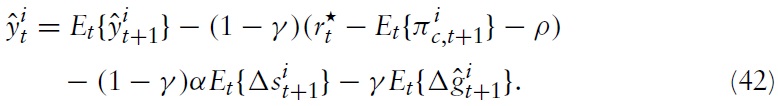
By using results from the utility-maximizing behavior of households, one can noweasily derive one of the key equations inNKmodels, the dynamic IS equation (or DIS, for short). First, we consider the home economy in country

Combining this expression with equation (38) yields the domestic DIS equation (approximated around a symmetric steady state):

This equation fully characterizes the demand side of country

3.4.2 Aggregate supply ? the New Keynesian Phillips Curve
The next task is to derive the second key equation that summarizes the dynamics on the supply side of the economy.
Note first that clearing the market for aggregate labor in country
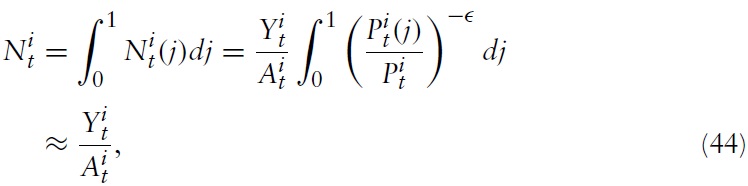
where the latter equations followfromthe production technology in equation (31) and the goods market-clearing condition in equation (36). The relation between output and employment in terms of deviations fromthe steady-state is thus simply given by:

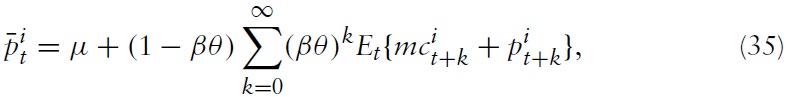
It can be shown that the profit-maximizing price-setting strategy, equation (35), can be manipulated such that one finally obtains an expression that determines the inflation dynamics in the economy. This equation is often referred to as the New Keynesian Phillips Curve (or NKPC, for short) and is given by

where λ ≡ (1 −

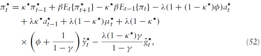
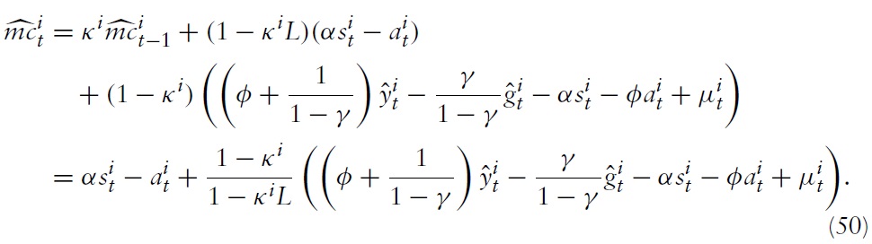
denotes the log deviation of marginal cost from its steady-state value. Inflation thus results from aggregate firms’ price-setting decisions, which in turn are determined by current and expected marginal costs. Accordingly, it makes sense to analyze the cyclical behavior of marginal costs. For this purpose, I derive a relationship between economy’s marginal costs and key variables measuring aggregate economic activity.
Note first that one can write marginal costs in equation (34) as

This can be combined with equation (23) to produce

From equation (48), it can be seen that an increase in productivitymust lead either to an increase in real wages or terms of trade or to a decrease in marginal costs. As will be evident later, depending on how policy is conducted, the outcome is either reflected in output or inflation.
Combining this expression of marginal costs with the partial-adjustment real wage equation in equation (28) and the

in equation (18), one gets:
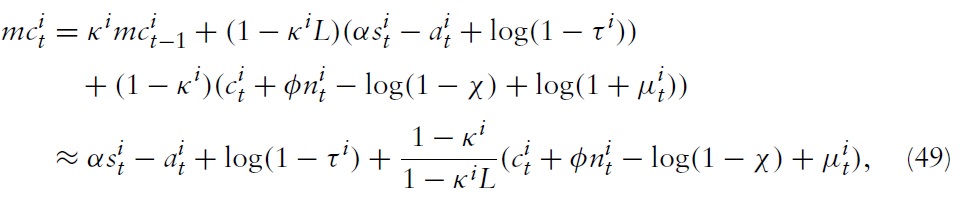
where
Expression (49) suggests that a higher real wage rigidity indicates a higher inertial adjustment of marginal costs. This is in line with empirical evidence. In a seminal paper, Galí
In order to express the latter equations in terms of deviations from the steady state, we make use here of equations (38), (45) and the fact that

Clearly, a cost-push shock increases marginal costs; however, the positive effect dies out if
Interestingly, there is a negative relationship between public spending and marginal costs. To give an intuition for this result, consider the implications from the aggregate market-clearing condition in equation (38): given the output, an increase in government spending crowds out domestic consumption and/or decreases the terms of trade; that is, it generates real appreciation. Both tend to have a negative effect on the

and thus, depending on
Because marginal costs feed into the determination of prices through the NKPC, we establish a direct channel of real wage rigidities to translate into the aggregate inflation of country
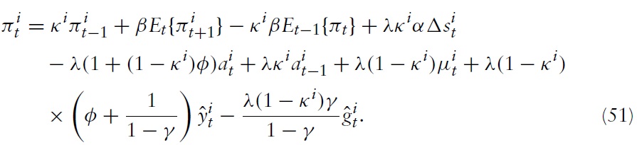
Integrating this expression over all member states yields the NKPC for the union as a whole, namely

where

for all
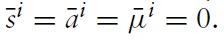
So far, I have derived log-linear equilibrium conditions for inflation and output according to the definition above. I have shown that the equations describing the equilibrium behavior of our economy can be summarized by just two equations. Given a function for government spending and a nominal interest rate characterizing the monetary policy, the equilibrium is determined for each individual economy by equations (42) and (51) or for the union as a whole by equations (43) and (52).
4One also could have introduced real money balances as an argument.However, if it enters additively (as empirical evidence suggests, see Ireland, 2004, for the case of the US, and Andrés et al., 2006, for the case of the EMU), a money-market equilibrium plays no role for the dynamics when the nominal interest rate is the monetary policy instrument. Therefore, money is ignored in the remainder. 5The assumption of exogenous variation in the markup is two fold. First, it keeps an already rich model clear and tractable. Second, it can be interpreted more generally as a cost-push shock. Of course, variations in wage rigidity could be an endogenous source for variation in the markup, but I abstract from this to draw more general conclusions. 6Equation (25) only holds under the assumption of symmetric initial conditions and initial zero net foreign asset holdings. For a detailed derivation of this result, see Galí and Monacelli (2008). 7As shown in Blanchard and Galí (2007) a more complex model with staggered real wage setting would lead to similar conclusions. 8Generally, one would want to guarantee that the real wage exceeds the MRS at all times in order to prevent workers from working more than desired, given the wage. For this reason, we consider the real wage in country i from the household’s perspective, i.e. and not the real wage in terms of the producer price index given by 9For instance, Brulhart and Trionfetti (2004) find evidence for (strong) home bias. 10Note that the efficient allocation is similar to the one in Galí and Monacelli (2008). Of course, real rigidities do not affect the social planner’s problem at all, nor does a markup shock affect the steady state of the model. Moreover, given that the labor demand function represents no additional constraints for the social planner’s problem. 11Note that denotes the realwage in terms of the (log) producer price index As mentioned above, I differentiate between producer and consumer price indexes; i.e. the (log) real wage from the consumer’s perspective is given by 12This result has, for instance, been shown in Galí (2008). 13This result follows directly from Galí and Monacelli (2008). As no expansion of the present model affects the steady state, it is similar to the one in this reference paper.
4. Calibration and Implementation
In the following numerical analysis of the model, we assume that time is taken as quarters.We set the discount factor

In order to solve the system of linear rational-expectations equations with lagged expectations, we follow the numerical procedure proposed by Meyer-Gohde (2010) but add some computational extensions. Basically, this approach is based on the method of undetermined coefficients for the infinite MA representation.
5.1.1 Member country’s trade-off
In a previous section, we derived a dynamic equilibrium in terms of real (aggregate) variables. In order to better interpret the business-cycle behavior of the economy from a welfare point of view, we further use the conventional notation of gap variables. That is, from now on we consider the deviations of the actual economy’s variables from the welfare-optimal level (i.e. the outcome in a Pareto-efficient allocation). That is, smaller gaps indicate smaller welfare losses.
To rewrite the equilibrium equations derived above, in terms of gap variables, note first that the deviations of marginal costs in a flexible price/wage setting from its efficient steady-state are given by

for all
Next,we define

as the output gap and the government spending gap, respectively. Moreover, I define a measure for the fiscal stance:

which I will refer to as the fiscal gap. Using these definitions and imposing an optimal steady-state government-spending share (
Because domestic policy depends on union-wide decision making, one can combine equations (39), (40) and the fact that inflation differentials that support an efficient allocation are inversely proportional to productivity growth differentials14 to obtain an equation that determines the output gap differentials in terms of fiscal gap differentials and changes in inflation differentials:

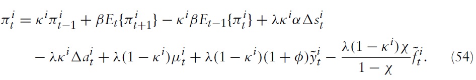
The previous two expressions describe the dynamics of the domestic price level, the output gap, and the fiscal gap, given the aggregate variables determined by union-wide policy.
It is directly seen from equation (54) that a positive markup shock inevitably puts some pressure on the domestic price level, which could only be absorbed by fluctuations in output (if no fiscal gap is created).The domestic authority will thus necessarily face a trade-off. The upward pressure on domestic prices decreases with

Depending on the inertia of the adjustment process, this affects the realwage paid by firms and thus affects marginal costs and thereby firms’ price-setting behavior.
While the trade-off due to a markup shock is simple and easy to grasp, the one resulting from a shock in technology is a little more complex. The latter two equations make clear that the trade-off is twofold. Consider first the situation in which real wages are fully flexible, that is,
Things differ substantially if real wage rigidities are present. It is easily seen from equation (54) that closing the output and fiscal gaps at all times no longer implies full price-level stability, even if shocks are purely symmetric. To understand the basic source of this trade-off, consider again the economy’s factor-price frontier in equation (48). Note that under flexible wages, a sudden shift in domestic productivity leads to an increase in real wages. If real wages are sticky, a shock in domestic productivity also leads to a decline in marginal costs.15 Obviously, greater sluggishness in the realwage indicates greater decreases in marginal costs.
It is seen in a previous section that the NKPC provides a direct channel for marginal costs to translate into the aggregate domestic inflation. The dynamic relationship implied by equation (46) makes clear that as marginal costs decrease, the price level experiences greater (downward) pressure. From equation (54) it follows that increasing pressure on the price level (and thus on the terms of trade) can only be absorbed by a decline in output relative to its efficient outcome (and/or by creating a positive fiscal gap).To conclude, in the presence of realwage rigidities in country
Furthermore, equation (54) implies that, given
5.1.2 Union-wide trade-offs
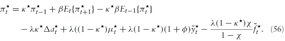
In order to derive the implications for union-wide policies, we integrate equation (54) over
Secondly, one can use equation (43) to derive an expression that determines the union-wide output gap:
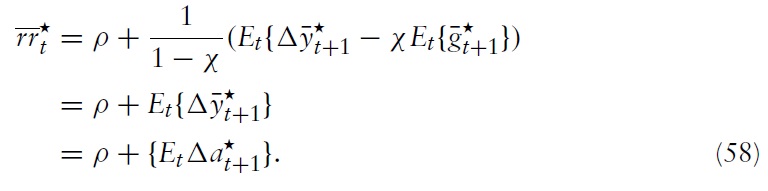
where

is the natural rate of interest, given by:
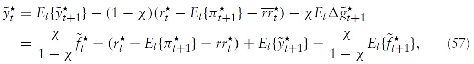
The NKPC in equation (56) and the DIS equation in equation (57) now fully describe the dynamics of aggregate inflation and the output gap, given a monetary policy rule in the form of a nominal interest rate and a fiscal policy determining the fiscal gap for all member states.
Because each member country is assumed to be of measure zero, a domestic shock has no effect on union-wide dynamics. Consequently, closing union-wide gap variables is always feasible (and optimal) and goes along with a constant aggregate inflation.
Of course, if shocks are not idiosyncratic, the conclusion differs substantially. Again, the trade-off resulting from a union-wide markup shock can be easily explained by considering the union as a closed economy: an increase in aggregate households’ market power leads to an increase in the union-wide real wage, depending on the rigidity, and thus to an increase in marginal costs on the firms’ side and thus in the union’s price level.
While a cost-push shock is a well-known source of a trade-off between stabilizing inflation and welfare-relevant output in NK models, a shock to technology is usually not. From equation (56), it is directly seen that, given the standard assumption of flexible real wages (i.e.,
5.2 Optimal Monetary and Fiscal Policy Design
The aim of this paper is to derive optimal monetary and fiscal policy rules for a currency union. Optimality is measured in terms of aggregate welfare. That is, a union-wide monetary policy and domestic fiscal policies seek to maximize aggregatewelfare (or minimize aggregatewelfare losses). In otherwords, I assume that all political authorities in the currency union act in perfect coordination with the best interests of the union; that is, national governments do not use their fiscal instruments to pursue policies in favor of domestic interests. 17 As welfare is defined as the aggregate household utility, the policymakers’ (perfect coordinated fiscal and monetary authorities) joint objective is similar to the one in a union-wide social planner problem18 and they will choose the same efficient steady state. The only difference is that political authorities are subject to the equilibrium conditions for any individual member country, as discussed above. In the following, I derive optimal policies for domestic and union-wide authorities under full commitment and full coordination.
As the analysis is based on gap variables instead of real variables, a welfare objective based on

for all
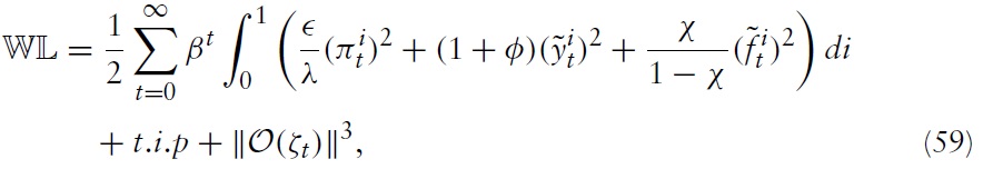
where
are terms of higher order.
There are several important qualitative features, which are evidently seen from equation (59). The welfare cost of variation in the price level is increasing with the substitutability across varieties produced within any country and the average duration of prices. Note that a rise in the price level in, say, country
Moreover, it can be perceived that the cost of output deviation from itswelfareoptimal level is decreasing with the labor-supply elasticity, that is, 1/
As mentioned above, the policy makers’ task is to minimize the welfare losses for all member states

Minimizing the appropriate Lagrangian with respect to

for all


where

denote the discounted Lagrange multipliers associated with the constraints in equations (54), (55), and (60).
5.2.1 Union-wide equilibrium dynamics under the optimal policy
In order to derive the implied path for
one can integrate equation (61) over

Similarly, integrating equation (62) over
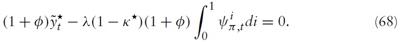
Now, by combining the latter two equations, one can derive a monetary policy rule that specifies a condition to be fulfilled by the central bank’s target variables:

for all
for

for
The optimal targeting rule for the monetary policy derived above implicitly assumes that the central bank can choose its desired level of inflation, output gap, and fiscal gap. Of course, in practice, the policy maker cannot set all three target variables simultaneously. One possibility to achieve the desired outcome is to set its policy instrument, namely the nominal interest rate, such that the optimal allocation is achieved.
By combining equations (57), (69) and (70), it can be seen that in the welfareoptimal equilibrium the nominal interest rate then equals

for all

and

A helpful exercise to draw explicit conclusions for monetary policy is to compare the optimal rule with actual policy conducted by the ECB. As a benchmark for actual policy, we use a standard Taylor-type rule estimated for the EMU. The Taylor-type rule takes the form

which is similar to the one used in Mattesini and Rossi (2009). Of course, in the Taylor-rule scenario, fiscal policy remains an invalid instrument for stabilizing the aggregate economy; that is, we assume equation (70) holds.
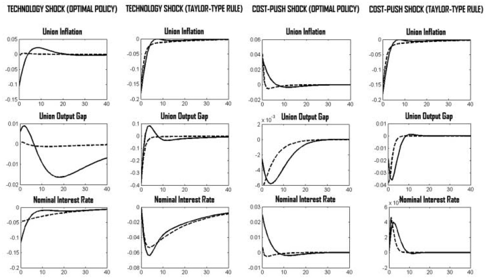
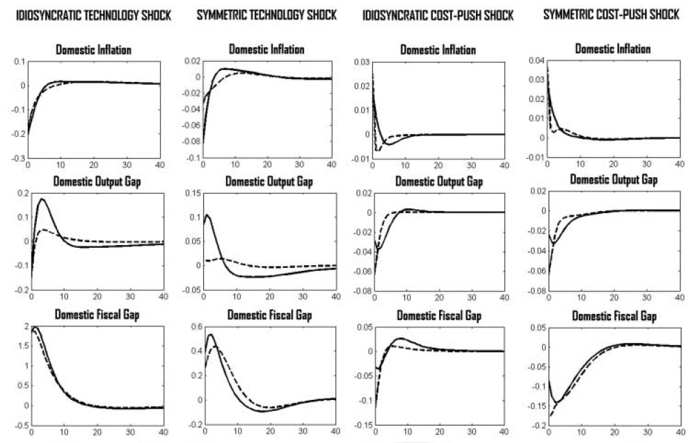
The IRFs of the optimal rule and the Taylor rule, in the face of symmetric shocks, are considered in Figure 1. It is seen that under both policies, fluctuations in the union-wide price level and aggregate output are increasing with real wage rigidity. The reasons are discussed in section 5.1.2. Moreover, both policy rules lead to qualitatively similar dynamics.However, since the Taylor-type rule is strictly backward looking, policy reacts with some delay compared with the optimal policy. Additionally, the optimal policy seems to put relatively more weight on reducing the output gap, while the Taylor rule focuses relatively more strongly on price-level stability.
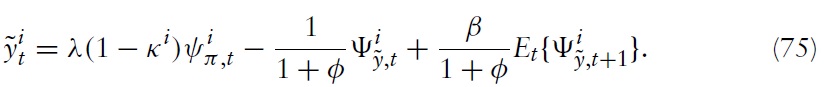
5.2.2 Domestic equilibrium dynamics under the optimal policy
In this section, the paths of inflation will be derived, along with the output gap and fiscal gap in a member state as implied by the optimal policy derived above. For this purpose, note first that equation (65), together with equation (66), can be written as

Combining equation (62) with equation (63) and using the latter expression yields:

Reconsider that the NKPC for each member state is derived fromits basic version in equation (46). This makes clear that equation (54) is a binding constraint for the optimization task as long as λ > 0 and thus as long as

is a positive number strictly greater than zero. From this, it follows that under the union-wide optimal policy, neither

nor

remains at its efficient level (this is also the case if real wages are fully flexible).
Next, I derive a dynamic equilibrium of the domestic economy in country

where

Note that the aggregate multiplier must evolve exogenously from country i’s perspective; the equilibrium relationship thus holds for any value of

Similarly, combining equation (62) with equation (65) yields
Finally, equation (63) together with equation (66) can be written as

Now, we can define a rational expectations equilibrium under union-wide optimal policies for country
for all
Note that this description of a rational expectations equilibrium is only valid if, and only if,

and, when combined with equations (54) and (55), describes the equilibrium dynamics of the domestic economy, given flexible prices.
The equilibrium dynamics for country
Consider first the case where only the domestic economy is hidden by a shock. Of course, any exogenous variation puts the domestic price level under pressure, as neither prices nor wages can adjust directly. Therefore, to the extent that the price level reacts gradually, a shift in productivity will be absorbed by a combination of a fall in the output gap and a rise in the fiscal gap. As discussed in a previous section, a higher real wage rigidity leads to a greater downward pressure on the price level in the face of a technology shock. Consequently, the expansion in output also has to increase to dampen the additional disinflationary pressure. Expanding the fiscal gap is necessary to bring about some demand to accommodate the desired expansion in output.
In contrast, towork against the inflationary pressure resulting from an increase in households’ market power, the optimal policy requires a decline in output. Because the initial pressure on the price level decreases with
However, if shocks are symmetric, domestic fiscal policies are not needed to adjust cross-country inflation differentials; theymust only absorb the pressure on the price level due to real wage rigidities. This is a crucial insight of this model and an important implication for optimal policy design in the EMU.
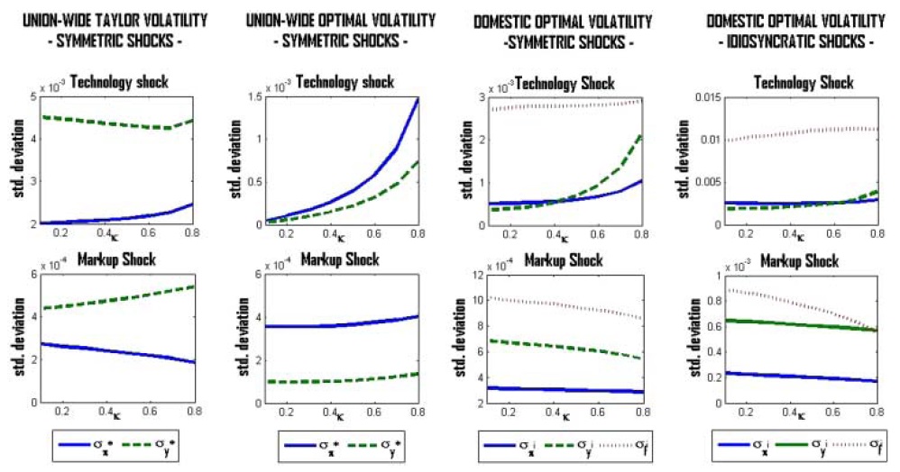
5.2.3 Optimal volatility
The analysis so far provides some advice for conducting policy optimally in the presence of real wage rigidity. Studying union-wide dynamics, it is seen that a higher realwage rigidity leads to a greater impact on inflation and output in all scenarios considered. In particular, the variability of inflation, contradicts (to some degree) the actual policy of the ECB, which emphasizes price-level stability as a central goal. In order to drawmore explicit conclusions on the quantitative importance of realwage rigidity in determining the deviation of the optimal policy from a policy aimed at attaching greater importance on price-level stability, a closer look at the optimal variability of the target variables is helpful. Figure 3 shows simulation-based computations of the optimal volatility of inflation, output, and the fiscal gap for different values of real wage rigidity.
Not surprisingly, the volatility of aggregate inflation and the aggregate output gap increases with real wage rigidity; therefore, the incentive for the common central bank to deviate from a strict inflation target should be higher. Moreover, optimal inflation volatility on the aggregate level is always higher (and increases more steeply with
Optimal volatility analysis on the domestic level also confirms the results found in the previous section. As expected, the optimal fluctuations in output at the national level are higher than those in price (at least for a reasonable degree of real rigidity). Furthermore, total volatility is higher (lower) in the event of an idiosyncratic technology (markup) shock.
14That is, The derivation of this result can be found in Galí and Monacelli (2008). 15This is because domestic authorities cannot avoid that the terms of trade adjust inefficiently. 16Basically, the implications for the union as awhole are closely related to those of a closed economy studied in Blanchard and Galí (2007). 17Forlati (2007) analyzes the case of non-coordination in a basic multi-country model of a currency union. 18This is because there are no (static) distortions in the steady state, given that the subsidy is set correctly.
In this paper, we investigate the consequences of real wage rigidities for optimal fiscal and monetary policy in a framework of a multi-country NK model of a currency union, where monetary policy is implemented throughout a union by a single central bank, and the fiscal policy is left to domestic authorities. We use shocks to productivity growth and wage-markup shocks in order to analyze the equilibrium dynamics of the domestic and union-wide economy.We assume that a domestic policy decision has no impact on other member countries and thus on the (aggregate) union-wide economy. As a consequence, one has to sharply distinguish between idiosyncratic and symmetric shocks. Considering the first scenario,we find that only the domestic country’s authorities are facing a trade-off between stabilizing output around potential and inflation. In the second scenario, the common monetary authority also faces a trade-off between stabilizing the aggregate price level and the welfare-relevant output.
As marginal costs feed into the determination of prices through the NKPC, we establish a direct channel of real wage rigidities to translate into (aggregate) inflation dynamics. It is shown that any considered exogenous variation puts pressure on the (aggregate and domestic) price level, as firms’ marginal costs cannot adjust efficiently. It is found that rigid real wages indeed provide evidence for inflation inertia.
We derive optimal monetary and fiscal policy from a union-wide perspective in the form of targeting rules. This is done by maximizing the aggregate welfare of the union. We thereby assume the full commitment and perfect coordination of the monetary and fiscal authorities, as the common objective is to maximize union-wide welfare. To approximate a welfare objective, a pure quadratic loss function is used,which approximates thewelfare losses associated with variations in the target variables. While fiscal policy cannot be used to stabilize the aggregate economy, common monetary policy does. Optimal monetary policy suggests that if nominal and real rigidities are present, and a shock is common to all member countries, the central bank stabilizes union-wide economy via a slightly countercyclical policy to dampen the pressure on the (aggregate) price level. The countercyclical activity increases with the importance of real rigidities. Compared with an estimated Taylor rule for the EMU, I find that optimal monetary policy should allow for higher inflation volatility relative to output volatility.
The role of fiscal and monetary policy is reversed at the national level. The reason is twofold. In the presence of idiosyncratic shocks, domestic authorities cannot avoid that the terms of trade respond inefficiently (because of the impossibility of resorting to nominal exchange rate adjustment), nor can they evade the (dis)inflationary pressure due to real rigidities. Reducing the pressure on the price-level variations in output is needed, and this must be induced by fiscal measures. Consequently, national fiscal policy is also justified as a stabilization tool from a union-wide perspective. However, if shocks are symmetric, inflation differentials do not provide a rationale for a countercyclical policy; only the sluggish adjustment of real wages does so. Again, the pressure on the price level has to be absorbed by a change in output. To create this output gap, the national government has to bring about or cut the necessary demand. In addition, at the domestic level, the importance of governmental intervention depends crucially on the degree of real rigidity.
Of course, the present model used for policy analysis is an abstraction of the realworld. Many essential features are not yet included, as there is always a tradeoff between tractability and realism. Some aspects seem likely to be relevant for the design of policy.We abstract from the need to rely on distortionary taxes, the effects of government debt policies, and the likely existence of incomplete Ricardian behavior on the part of households. Moreover, by relaxing the assumption of perfect risk sharing, one could possibly generate a complementary role for fiscal policy as a cross-country insurance tool. Further research is necessary to include more features related to reality.