Two of the most important trends in the global economy in recent decades have been (1) the dramatic increase in the role of information-intensive products (e.g., various types of computer software products, consumer electronic products and IT-related services), and (2) the proliferation of trade liberalization through both economic integration and preferential trade agreements. Advances in both digital technology and trade liberalization have driven an increase in the flow of information-intensive products across countries.1

As a result of these changes, consumers face an international array of competing product groups based on incompatible, proprietary standards.2 The choices among computer operating systems, television broadcasting standards, and DVD systems are recent examples. In addition, it is widely recognized that products based on the same industrial standard exhibit an indirect network effect: the utility of consumers is increasing in the variety of complementary products based on a particular standard.3 Trade liberalization matters in this context because it reduces import prices, and changes (usually enlarges) the available sets of complementary products, thus influencing a society’s patterns of consumption.

In such settings, competition between a ‘domestic’ standard and a ‘nondomestic’ standard is often observed. A recent example is the global competition among wireless telecommunications service providers. Funk (1998) suggests that, although most service providers are likely to dominate domestically and thereby make the ‘home’ standard dominant, firmssuch as Motorola, Ericsson, and Nokia have succeeded in marketing a ‘non-domestic’ standard. He suggests that, while Motorola USA’s market share in Europe is lower than in its domestic market, it still holds a significant position in the European (and therefore theworld) market.4 Another famous example involves incompatible color television standards. It is widely believed that incompatible standards for color television (i.e., the NTSC system in the US and Japan; the PAL system inWestern Europe) have contributed significantly to Japanese firms’ lower market share in Western European markets relative to the US market.5 There seems to be a case for closer examination and more formal modeling of increased trade in technology-related products and fiercer competition among incompatible industrial standards.

In the literature on trade and competing industrial standards, the role of government standardization policy is often emphasized. In their influential contribution, Gandal and Shy (2001) analyzed governments’ incentives to recognize foreign standards when there are potentially both network effects (i.e., consumption benefits) and conversion costs. Their focus was on how standardization policy affects both international trade flows and national welfare.

An important question about the relationship between competing industrial standards and trade liberalization remains unanswered: how does trade liberalization affect consumers’ choice between incompatible standards? The main  purpose of this study is to illustrate, with simple trade theory, this relationship. Following Matsuyama (1992), we assume that there are two incompatible standards, each of which applies to a group of differentiated products. A product can be used only in combination with other products based on the same industrial standard. Matsuyama assumed a closed economy and paid scant attention to the role of trade liberalization. In contrast, in this study we focus on the case of competing industrial standards in an international context (i.e., a Home standard and a Foreign standard) and examine the impact of trade liberalization (i.e., a decline in trade costs) on consumers’ choice of a standard.

The structure of this paper is as follows. In the next section we present a basic model: assuming that products are only consumed in a single (i.e., Home) country,we consider the competition between the Home standard and the Foreign standard. Based on this basic model, in Section 3, the impact of unilateral trade liberalization (i.e., a decrease in trade cost on Foreign products in the Home country) is considered. In Section 4, we extend the basic model to the case of twosegmented (i.e., Home and Foreign) markets, and the impact of bilateral trade liberalization is considered. Concluding remarks are presented in Section 5.

1Addressing this point, the OECD (2006: Ch. 2) reports that between 1996 and 2004 the annual increase in OECD countries’ exports of ‘software goods’ was 5%, while imports increased by an average of 6.5% per year.   2In this study we will use the term ‘standard,’ not in the sense of government regulation, but in the universal sense of the set of technical specifications that enable compatibility among products.   3The seminal contributions on the indirect network effect are by Chou and Shy (1990) and Church and Gandal (1992). See Gandal (2001, 2002) and Farrell and Klemperer (2007) for surveys of the relevant literature. In the international context, see Iwasa and Kikuchi (2008) and Kikuchi (2005, 2007) for analyses of trade liberalization in the presence of network effects.   4Motorola’s share of the world market dropped from 40% in 1994 to 32% in 1995, as use of the European GSM standard grew. Still, it is larger than Nokia’s share in the world market (22%). See, also, Lembke (2002).   5Burton and Saelens (1987, p. 291) note that, while sales by Japanese firms accounted for 43.5% of all sales in the US market in 1981, Japanese firms held only a 15.2% share of theWestern European market in 1983. (Note that the Japanese televisions that are exported to the Western Europe are based on PAL system.) Rohlfs (2001) discusses this in terms of network effects.

Suppose that there are two countries, Home and Foreign. In this and the next section, we concentrate on what happens in the Home market. Both Home firms and Foreign firms compete in the Home market, which is defined as a line of unit length representing consumers’ set of preferences. Home consumers are indexed by z, z∈[0, 1], and with no loss of generality, we normalize the total mass of Home consumers to equal 1. Each consumer is endowed with the amount E of income to be spent on differentiated products.

Assume that there are two competing industrial standards: Home standard and Foreign standard. A variety of differentiated products can be produced based on either standard: we simply assume that Home (resp. Foreign) firms produce products based on the Home (resp. Foreign) standard. The two standards are not compatible with each other, hence any product can be used only in combination with other products based on the same standard.6

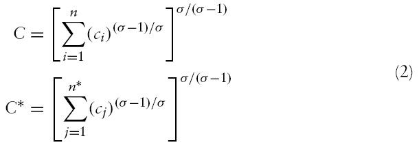
Each consumer is assumed to purchase products based on only one standard (Home or Foreign). We call the two groups of differentiated products Home standard products and Foreign standard products. The utility of consumers is  assumed to be increasing in the variety of complementary products based on a particular standard. We define the utility of an individual of type z by

where C (C^∗) is the quantity index of Home (Foreign) standard products. These indices are defined in the Dixit-Stiglitz (1977) form

where n (n^∗) is the number of Home (resp. Foreign) standard products and σ >1 is the elasticity of substitution between every pair of products, within the same standard.

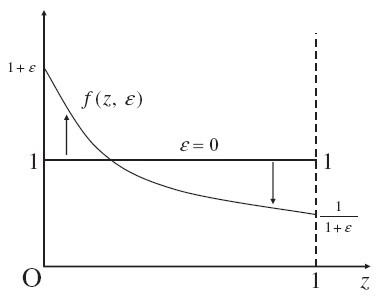
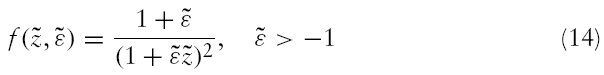
Following Chou and Shy (1996, p. 314), we assume that the density function of consumers’ types is given by,

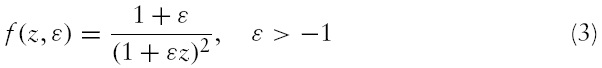
when ε=0, the density function becomes uniform, representing the case in which consumers are evenly distributed on [0, 1]. Figure 1 shows that when ε increases, the distribution shifts towards the Foreign standard.When −1<ε<0, the distribution is biased in favor of the Home standard.

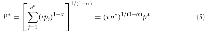
The importation of Foreign products is inhibited by frictional trade barriers, which are modeled as iceberg trade costs: for 1 unit of Foreign product to reach Home, t ∈ (1,∞) units must be shipped. Thus, the price of an imported product to Home consumers will be tp^∗, where p^∗ is the producer’s price for Foreign standard products. It is important to note that this trade cost includes all impediments to trade such as tariffs, but also communication difficulties, information barriers and cultural differences. Price indices for each group of standard products, which indicate costs for obtaining one unit of quantity index, are defined as follows:

where τ ≡t^1−σ ∈(0, 1) is the measure of the freeness of trade, which increases as t falls and is equal to one when trade is costless (t=1). Note that τn^∗ represents an effective number of Foreign standard products: trade liberalization (i.e., a larger τ) can be interpreted as an increase in the number of varieties even if n^∗ remains unchanged.

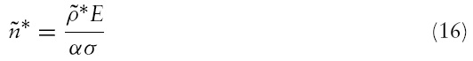
Let us turn to the cost structure of differentiated products. In order to simplify the argument, technology is assumed to be identical between countries and characterized by increasing returns to scale, since both product creation and market entry typically involve fixed costs.7 We denote the constant marginal cost of production for every product by β, and the fixed cost by α.8 We assume that firms are monopolistic competitors. Given a Dixit-Stiglitz specification with constant demand elasticity σ, each firm chooses its constant markup price as

Let us denote the number of consumers who purchase Home (resp, Foreign) standard products as ρ (resp. ρ^∗). Note that ρ + ρ^∗=1. Then, assuming that the entry and production decisions of the potential firms cannot individually affect the existing firms, the equilibrium number of products produced according to each standard becomes proportional to the total expenditure on products based on each standard:

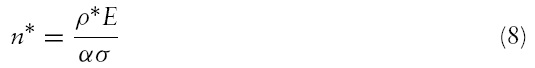
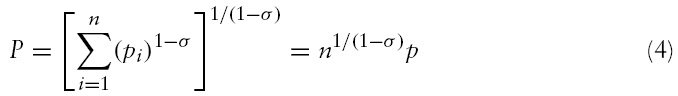
Combining equations (4), (5), (7), and (8), it can be easily shownthat a consumer’s welfare increases when more consumers purchase products with the same standard. As more consumers choose the same standard, more firms choose to produce based on that standard. This results in increased product diversification among products with that standard.

This results in the types of ‘indirect network effects’ analyzed by both Chou and Shy (1990) and Church and Gandal (1992): network effects work indirectly via increased diversification of products (see Gandal, 2002).

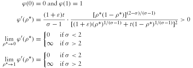
Now let us turn to the equilibrium number of consumers who purchase Home/Foreign standard products. We denote by

the type of the marginal consumer who is indifferent between two standards. Using equation (1),

is derived as

The equilibrium number of consumers who purchase Foreign standard products, ρ^∗, can be obtained by integrating the density function (3) from 0 to

as follows:

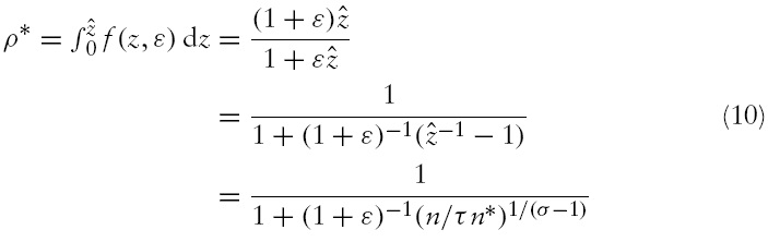
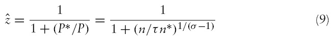
Substituting in the equilibrium number of differentiated products, we can obtain the equilibrium proportion of consumers who purchase Home standard products:

6See Matsuyama (1992) for elaboration on this point. This assumption implies that, for one country’s producers, the cost of converting to the other standard is extremely high. Although this assumption is restrictive, it is often argued that the existence of (high) conversion costs affects foreign firms’ behavior (Gandal & Shy, 2001).   7As a first step to incorporate competition between industrial standards, we will concentrate on the case of identical technology between standards. In order to analyze the interaction of technology gap and standard competition, an extension for asymmetric technologies needs further consideration.   8For discussion on the role of market entry in the presence of fixed costs, see Melitz (2003).

In this section we consider the impact of unilateral trade liberalization (i.e., a reduction in t in the Home market). From equation (11), we can obtain the equilibrium relationship for the number of consumerswho purchase Foreign standard products:

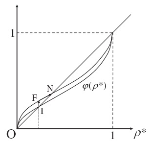
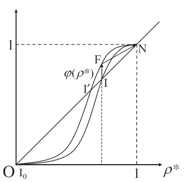
Figures 2 and 3 help to illustrate the trading equilibrium. The curves represent ϕ(ρ∗) functions, which show the possibilities for the number of consumers who purchase Foreign standard products that are consistent with firms’ entry/exit decisions. The trading equilibrium is obtained as the intersection between these curves and the 45° line. From the ϕ(ρ^∗) function we can obtain the following:

These results indicate that, depending on the level of elasticity between varieties, σ, one of two cases will emerge. We shall discuss each case in detail.

First, it is important to note the multiplicity of equilibria. Clearly from Figures 2 and 3, there are three possible equilibria in each case: two corner solutions (only Home (or Foreign) standard products exist) and an interior equilibrium where both standard products coexist. If the economy initially stays at the corner solution, a reduction in trade costs does not affect the equilibrium configuration. Thus, in what follows, we concentrate on the interior equilibrium  where both standard products initially coexist.

When σ >2 holds, the indirect network effects are relatively mild. The initial trading equilibrium is obtained as point I in Figure 2. Trade liberalization implies an increase in the effective number of Foreign varieties, τn^∗, which makes Foreign standard products more attractive: this change is shownas an upward shift in the ϕ curve. Since some consumers who had been purchasing Home standard products switch to Foreign standard products, more Foreign firms enter intoHomemarkets. The new equilibrium is obtained as point N on the 45° line.

The point is that there is a cumulative process in which trade liberalization will enhance Home consumers’ propensity to switch to the Foreign standard, and this switching will induce further product diversification among Foreign products.  Still, since the indirect network effect is mild, some consumers who prefer Home standard products continue to choose those products.

This result is also quite important from the welfare perspective: since trade liberalization leads some Home consumers to ‘switch’ to the Foreign standard, the market size for Home standard products will shrink and consumerswho continue  to choose Home standard products are made worse off by trade liberalization.

It is important to note that the result that some consumers are made worse off by trade liberalization is not newin trade literature as Heckscher–Ohlin and other competitive models show. However, our results are derived from an imperfectly competitive setting.

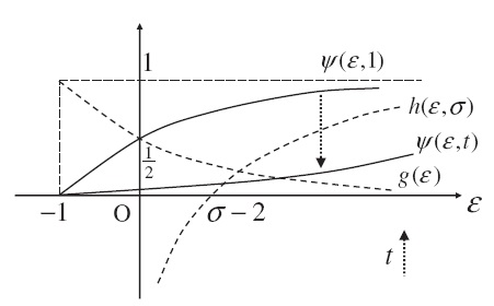
Next, let us consider the changes in total consumers’ welfare, which is defined as follows:

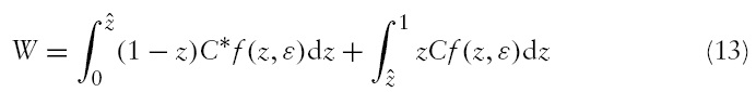
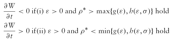
Differentiating W with respect to t, we obtain sufficient conditions under which trade liberalization makes total welfare of Home consumers better or worse off.

where

and

Proof. See the Appendix for the proof.

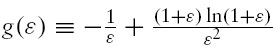
Figure 4 helps to illustrate the relationship between g(ε), h(ε, σ), and ρ^∗=ψ(ε, t).9 The horizontal axis indicates ε, while the vertical axis indicates the values of each function.10

Proposition 3 (condition (i)) implies – given that the Home consumers’ preferences are biased toward Foreign standard products and the initial share of Foreign standard products is sufficiently large – that trade liberalization increases total Home welfare. Thus, although some consumers who continue to choose Home standard products will be made worse off by trade liberalization (Proposition 2), one can find a redistributive scheme that makes nobody in Home worse off. As space is limited, we have concentrated on the changes of total consumers’ welfare and paid scant attention to the redistributive scheme.11

When 2>σ >1 holds, consumers’ valuation of product varieties (i.e., the degree of indirect network effects) is relatively high. Under this setting there are multiple equilibria: (2a) the stable equilibrium with no Foreign standard product; (2b) the unstable equilibrium with coexistence of both standard products; and (2c) the stable equilibrium with no Home standard product. Let us examine case (2a) and case (2b) separately.12

In case (2a), the initial trading equilibrium is obtained as point I0 in Figure 3. In this case, although trade liberalization reduces the price of Foreign standard products, Home consumers continue to choose Home standard products. This is because of strong indirect network effects: consumers have a strong incentive to purchase a product with large product diversification.

This result is quite important for considering the relationship between the level of trade costs and the amount of imports. For example, careful analysis of Japan’s trade volume during the 1980s suggests that Japan imports only about half as much as one would expect.13 Our result suggests that, given the existence of strong indirect network effects, one country’s consumers may stick with their own country’s standard products even though trade is liberalized.

In case (2b), the initial trading equilibrium is obtained as point I in Figure 3.14 An increase in the effective number of Foreign varieties has more influence than in the case with the previous subsection (i.e., an upward shift of the ϕ curve). Then consumers’ incentives to switch to Foreign standard products also become greater, which further induces Foreign firms’ entry. Then, the demand for Home standard products vanishes. The new equilibrium is obtained as point N on the 45° line.15 From Figure 3, one can obtain the surprising feature of the impact of trade liberalization.

A comparison between these three cases (1, 2a, 2b) highlights the important role of indirect network effects. On one hand, if the indirect network effect is mild, trade liberalization makes the Foreign standard more attractive to some  extent. Still, some consumers who prefer Home standard products continue to choose them. On the other hand, if the indirect network effects are sufficiently strong, the effects of trade liberalization are crucially dependent upon the initial  situation. Given that initially there are no Foreign standard products (2a), trade liberalization has no effects on trade flows. Instead, given the coexistence of both standard products (2b), trade liberalization will take Home standard products completely out of the Home market.

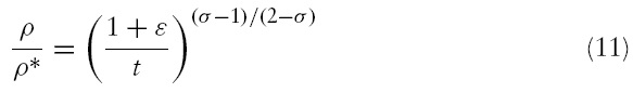
9From equation (11) we obtain    which gives the value of ρ∗ corresponding to the interior equilibrium. Note that limε→−1+0 ψ(ε, t) = 0, limε→∞ ψ(ε, t) = 1, ∂ψ(ε, t)/∂ε>0, and ∂ψ(ε, t)/∂t<0.   10Figure 4 indicates that, the smaller (resp. larger) t becomes, the higher the possibility of (∂W/∂t)<0 (resp. (∂W/∂t)>0) becomes.   11For this point, see, Kemp and Shimomura (2001) and Fujiwara (2005).   12In case (2c), since there are only Foreign standard products, trade liberalization does not change the nature of trade flows.   13See Lawrence (1987).   14It is important to note that point I is unstable. One interpretation of this situation is as follows: suppose that initially σ is sufficiently close to (but larger than) 2 for the point I to be stable. Then, some parameter change increases σ, which changes the slope of the ϕ curve. In this situation, at least initially, the economy might stay at point I. Thus, the results in case (2b) need to be interpreted with great caution.   15Another possible equilibrium is point I´. However, since potential Foreign firms enter due to improved access to the Home market and more consumers switch to Foreign products, it seems to be natural that point N will be selected as the new equilibrium.

Now consider the case markets with both a Home market segment and Foreign market segment.To simplify the argument,we concentrate on the case inwhich the degree of indirect network effects is mild (i.e., σ >2). As with Home consumers, the total mass of Foreign consumers

is normalized to 1.16 Assume that consumers’ taste in Foreign market is represented by equation (1). We assume that the density function of consumers’ types in the Foreign market is given by,

The only difference is the distribution of consumers’ tastes: since a larger value of ε implies the distribution is biased toward the Foreign standard product, we assume that

holds. In the Foreign market, the price of an imported Home standard product will be

while that of a (domestic) Foreign standard product will be p^∗. Furthermore, we assume that each firm must incur fixed costs to enter the market, α. Then the equilibrium number of products produced in the Foreign market is

where

is the number of consumers who purchase Foreign standard products in the Foreign market.

We should notice that the fixed market entry cost is market-specific: the producers of Home (resp. Foreign) standard products, which have been paid market entry cost for its own market, have to pay additional market entry cost when  they decide to export to Foreign (resp. Home) market. This implies that the numbers of Home and Foreign standard products in each market are determined independently

17

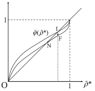
Following the same procedure as in the Home market, we can obtain the equilibrium relationship for the number of consumerswho purchase Foreign standard products in the Foreign market:

Figure 5 helps to illustrate the impact of bilateral trade liberalization. If both t and

become smaller, ϕ(ρ^∗) shifts upward, while

shifts downward. Thus, while the number of Home standard products becomes smaller in the Home market (i.e., n decreases), the number of Home standard products becomes larger in the Foreign market

This implies that the degree of intra-industry trade of non-domestic standard products will be increased by bilateral trade liberalization.

Let us consider this proposition more precisely. In each country, with the increased effective number of non-domestic standard products, consumers begin to switch to those products. Such switching will provide opportunities for the  entry of non-domestic standard producers.As with Proposition 1, the point is that there will be a cumulative process in which bilateral trade liberalization encourages consumers to switch towards non-domestic standard products, and those switchings will induce further intra-industry trade of non-domestic standard products.

16We use ‘∼’ to denote Foreign market values.   17This approach relates to that of Melitz (2003). In an alternative approach, one can assume that the fixed costs are paid only once. Then, the equilibrium number of products is obtained by adding both markets’ demand conditions. Although that approach is desirable, deriving explicit solutions from such a system of simultaneous equations might not be feasible. An extension for this setting needs further consideration. We would like to thank one referee for pointing this out.

Both trade liberalization and advances in digital technology have intensified competition between incompatible industrial standards. In this study, we explained the mechanism by which trade liberalization influences consumers’ choice of a standard. In Sections 2 and 3 we examined the impact of unilateral trade liberalization in a single (i.e., Home) market. It should be emphasized that the degree of substitution between product varieties plays an important role in determining the impact of trade liberalization: if the degree of substitution is sufficiently small (i.e., the indirect network effect is relatively large) and both standard products coexist before trade liberalization, trade liberalization will take Home standard products completely out of the Home market. In Section 4, we examined the impact of bilateral trade liberalization in a setting with two segmented markets. It was shown that the intra-industry trade of non-domestic standard products will be increased by bilateral trade liberalization.

This result (increased intra-industry trade due to trade liberalization) is not so new.18 However, we would like to emphasize that the cumulative process of consumers switching and firms enteringworks as a driving force behind the increased intra-industry trade. This point has not appeared in the existing literature.

The present analysis must be regarded as tentative. Hopefully, it provides a useful paradigm for considering how trade liberalization affects international competition among industrial standards.

18See, for example, Helpman and Krugman (1985).