A notable feature of the Mexican economy since the late 1980s was the persistent appreciation of the peso in real terms. For a small open economy, this is a key development. The appreciation not only makes exports less competitive – a drawback for a country pursuing an export-led growth strategy – but it also affects negatively profit margins, and hence investment, in the tradables sector (see Eichengreen, 2008, and Rodrik, 2008 for general analyses, and Ibarra, 2008a for evidence on the Mexican case). The appreciation thus helps to explain Mexico’s problem of slow economic growth.
The appreciation took place across different exchange-rate regimes (a crawling peg, a crawling band, and finally a float) but with the constant of a gradual process of disinflation. After a sharp reduction of inflation in 1989, and separated by the 1994–1995 economic crisis, there were two phases of gradual disinflation. In the first phase the annual inflation rate fell from 20% in 1990 to 7% in 1994; meanwhile, the Bank of Mexico’s real exchange rate index – a multilateral ratio of foreign to local consumer prices – fell from 119.1 to 90.4 (1988–2006 average = 100). In the second phase the inflation rate fell from 34% in 1996 to 5% in 2002, while the real exchange rate index dropped from 112.6 to 72.8. After the end of the second phase, the real exchange rate reversed, partially, its previous appreciation, reaching a level of 86.9 in 2006.
Despite the setting of prolonged disinflation, it has been frequently argued that the real currency appreciation was unrelated to the stance of monetary policy. In the mid 1990s the Mexican authorities insisted that the appreciation reflected the boost to productivity triggered by structural reforms (see for example Bank of Mexico, 1995). More recently, the appreciation has been attributed to large labor remittances and the high price of oil (see IMF, 2006). An exception is Galindo & Ros (2008), who argue that an asymmetric response of monetary policy to exchange rate changes contributed to the appreciation of the peso during the period 1995 to 2004.
Downplaying the role of monetary policy follows from the proposition that only real-side variables can have a lasting influence on the real exchange rate.1 But the neglect of monetary factors seems unsuitable in Mexico’s case, given the country’s prolonged disinflationary process and the overriding emphasis of monetary policy on that goal (see Ramos & Torres, 2005; Ibarra, 2008b). In fact, the episode provides an opportunity to study whether a sustained shift in monetary policy can have lasting effects on the real exchange rate.
The paper presents the results of an econometric study of exchange rate determination in Mexico. The study is based on the so-called BEER (Behavioral Equilibrium Exchange Rate) model, a model that jointly considers real-side and monetary determinants and that relies on Johansen’s cointegration methodology – a natural econometric framework to test for the existence of lasting or ‘longrun’ effects. The period under analysis starts in 1990Q1 (to focus on the period of free capital mobility in Mexico, as required by the risk-adjusted interest parity condition underlying the BEER model) and ends in 2006Q4.
The estimation results, in the form of two- and three-equation cointegration models, showsignificant long-run effects of monetary policy on the real exchange rate in Mexico; in particular, they show that – controlling for the influence of real-side determinants like the oil price, government consumption, and relative manufacturing production – a rise in the nominal interest differential appreciates the currency by two channels: directly, through a rise in the real interest differential; and indirectly, through a fall in the inflation differential.
The rest of the paper is organized as follows. Section 2 provides the macroeconomic background; section 3 briefly reviews the BEER model and the econometric methodology; section 4 presents the estimation results; and section 5 summarizes the paper. An appendix details the data sources and definitions.
1See Williamson (1994) for a discussion of the proposition, Kildegaard (2006) for an example applied to Mexico, and Frankel (2007) for a recent counter-example. The proposition does not imply, of course, that an appreciation caused by real-side variables, such as an oil windfall or a surge in foreign capital inflows, will not have negative growth effects, particularly in the tradables sector (see Krugman, 1987).
2. Real Exchange Rate and Macroeconomic Performance in Mexico
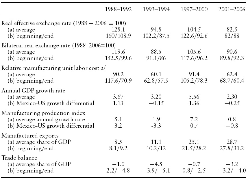
Table 1 presents selected indicators of macroeconomic performance in Mexico since 1988 – after the country liberalized its trade regime – averaged over periods that track the country’s growth cycle. The table includes three measures of the real exchange rate: the multilateral ratio of foreign to Mexican consumer prices; the bilateral ratio between the US and Mexico; and the relative unit labor cost in the manufactures between the two countries.2
Interrupted only by the 1994–1995 currency crisis and by the end of the second phase of disinflation in 2002, there is a clear tendency for the peso to appreciate in real terms. In addition, within this tendency it is possible to single out periods with relatively high (depreciated) exchange rate levels: 1988–1992 and 1997–2000, and periods with low levels: 1993–1994 and 2001–2006.
The fact that the three measures tell the same story is important. If the appreciation revealed by relative consumer prices merely reflected productivity growth differentials, the relative labor cost should be stable – which is not the case. For instance, while the multilateral ratio indicates an appreciation of about 21% between 1997–2000 and 2001–2006, the relative labor cost also indicates an appreciation, of about 32%.
The real exchange rate leads the growth cycle of the Mexican economy, both in absolute terms and relative to the US economy.3 In the periods with a depreciated currency, Mexico’s average GDP growth rate exceeds the US rate by more than one point; when the currency appreciates, the Mexican growth rate falls – both over time and with respect to the US rate. The pattern characterizes both the entire economy and the manufacturing sector.
Given the upward trend of the export share after trade liberalization, the simple averages of Table 1 cannot uncover the effect of the appreciation on manufactured exports. Moreover, the share of exports in GDP jumped after the enactment of the North American Free Trade Agreement in 1994 and the currency crisis of 1994–1995, almost doubling between 1994 and 1997. The table does show, however, that manufactured exports gradually lost dynamism, rising by only three points of GDP during 2001–2006.
[Table 1.] Selected macroeconomic indicators

Selected macroeconomic indicators
Lacking a trend, the ratio of the trade balance to GDP shows more clearly the possible influence of the real exchange rate. For instance, the average trade deficit rose from less than one point of GDP during 1997–2000 to more than three points during 2001–2006, despite the high price of oil. Since the Mexican GDP growth rate fell from 5.6% to 2.3%, the rise in the trade deficit cannot be attributed to an acceleration in economic growth.
2See Chinn (2006) for a discussion of alternative measures of the real exchange rate. 3The real exchange rate indices in Table 1 are lagged one year to better visualize their effect on macroeconomic performance.
What are the factors that explain the tendency of the peso to appreciate in real terms? The so-called BEER (Behavioral Equilibrium Exchange Rate) model provides a framework to test for the possible influence of both monetary and real-side variables on the real exchange rate. Moreover, for estimation purposes, the model relies on Johansen’s cointegration methodology, which seeks to detect lasting or ‘long-run’ effects (see Clark & MacDonald, 1998; MacDonald, 2007).4
The model is based on a risk-adjusted interest parity condition between domestic and foreign assets, which in nominal terms can be written as:

where

is the log rate currently expected for the end of the investment period,
The parity condition can be expressed in real terms by adding and subtracting the difference between the expected domestic and foreign inflation rates. Using the current difference as a proxy for the expected one, as is standard in the BEER literature, the result is:

where
Note that rather than including the real interest differential, equation (2) keeps its components – the nominal interest differential and the inflation differential – separated. This follows from the observation that, while the rest of the variables in the models have a unit root (see below), the real interest differential is stationary. If no further restrictions are imposed, the specification allows the estimated coefficients on the components of the real interest differential to differ in absolute value; this may be useful if, for instance, the unobserved risk premium responds to the inflation differential (for instance, because of Mexico’s problematic history with inflation control). In any event, the outcome of imposing symmetry on the estimated coefficients is explored at the end of section 4.
Equation (2) implies that the real exchange rate is positively related to the inflation differential and negatively to the nominal interest differential. The negative sign of the latter relationship is important for the correct interpretation of the estimation results. If there is fear of floating, monetary authorities may lean against the wind – that is, they may adjust the interest rate to stabilize the exchange rate (see Calvo&Reinhart, 2002) – making the interest rate ultimately depend on theexchange rate, rather than the other way around. Empirically, this would imply a positive relationship between the interest differential and the exchange rate – in contrast to the prediction from the interest parity condition. By supporting one interpretation over the other, the sign of the estimated coefficient can be used to settle the question.
Starting from the parity condition, the BEER approach consists of (a) positing a number of real-side determinants of the risk premium and the expected real exchange rate, and (b) estimating equation (2) by cointegration techniques. Following Kildegaard (2006) and Dabós and Juan-Ramón (2000), our analysis will consider three real-side variables: the ratio of Mexico’s manufacturing production index to the US index (RIMP, in natural logs), the international price of oil in real dollar terms (OIL, also in natural logs), and Mexico’s ratio of government consumption to GDP (GOVCOR).5
The manufacturing production ratio – intended to capture the Balassa–Samuelson effect – is a proxy for relative productivity in the tradables sector. A rise in relative productivity increases the consumer price index by its effect on wages and prices in the non-tradable sector, and therefore it is expected to reduce the real exchange rate. Under the assumption that it is biased toward non-tradable goods, a rise in government consumption should have the same effect.
The oil price is included on account of the large share of oil in Mexico’s nonmanufactured exports. There are several possible effects. Since a higher price of oil improves the current account balance, the real value of the peso must rise to keep the balance – and hence the country’s rate of debt accumulation – constant. Alternatively, a rise in the oil price produces a foreign-exchange windfall that pushes up the local currency. Finally, the windfall can increase the demand for non-tradable goods and raise the consumer price index.
Equation (2) was estimated following Johansen’s cointegration methodology (see Juselius, 2006, for a detailed presentation). The starting point is the following

where
There can be up to

where
The [
There are potentially six endogenous variables in our model: the bilateral real exchange rate,7 the interest and inflation differentials, the manufacturing production ratio, the oil price, and government consumption. Weak exogeneity tests indicate that the oil price can be considered as exogenous at 5% significance.8 In addition, there are reasons to consider government consumption also as exogenous. First, economic reasoning suggests that fiscal policy has a large discretionary component. Second, including the variable as endogenous yields poor estimation results: its coefficient on the real exchange rate cointegration equation is wrongly signed, while the coefficient on the manufacturing production ratio becomes non-significant (results available upon request).
For the above reasons, the oil price and government consumption are entered as exogenous variables. In the initial specification the models also include a constant, a linear trend, and a 0–1 CRISIS dummy for the first quarter of 1995 – although whether those variables remain in the final specification depends on their statistical significance and on the results of the LR test. The constant and trend are intended to capture other possible influences, such as the unobserved risk premium, on the endogenous variables.
4The definition of ‘long-run’ can be a matter of debate (see Driver & Westaway, 2004). In what follows, a long-run relationship is understood as a relationship in levels (as opposed to first differences) between the real exchange rate and its determinants within the specific horizon of 17 years of quarterly observations spanning 1990 to 2006. 5BEER studies usually include the country’s net foreign assets (NFA) position among the determinants of the real exchange rate. Since there are no readily available quarterly series for Mexico’s NFA position, one was constructed using the current account balance as a proxy for the change in NFA. The constructed series resembled closely the annual series presented by Lane and Milesi-Ferretti (2006); compared with the rest of the variables in the models though, it had a higher degree of integration, making its inclusion problematic. Following Fazio et al. (2007) the current account balance itself was considered as a proxy for NFA, but its estimated coefficient tended to have the wrong sign in the real-exchange-rate equation (a result also obtained by those authors). See Note 14 for the inclusion of government debt as a possible determinant of the risk premium. 6To avoid confusion, keep in mind that the number of cointegration equations in Johansen’s reducedrank regression methodology is always smaller than the number of endogenous variables in the VAR. 7While the series for the multilateral rate are available from the Bank of Mexico, the bilateral US–Mexico ratio must be used to be consistent with the peso–dollar interest differential. 8The LR test statistic was 5.65, with a p-value of 0.0592. Note that, somewhat surprisingly, the test would reject the (weak) exogeneity of the oil price at 10% significance, despite the oil price being determined in the world market with no influence from the Mexican economy. The weak exogeneity tests were carried out within an otherwise unrestricted cointegrated VAR, estimated under the assumption of two cointegration relationships (see trace test results below).
The risk-adjusted interest parity condition underlying the BEER model is an adequate description of assets market equilibrium only in a context of free capital mobility. Our analysis will thus be restricted to the period 1990Q1–006Q4,which roughly begins with the liberalization of the capital account in Mexico.
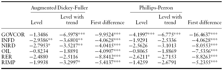
Table 2 presents the unit-root test results. In general, it is not possible to reject the hypothesis that the variables are non-stationary, and therefore that cointegration is the appropriate estimation framework. Table 3 presents the diagnostics for the original VARs, consisting of tests for normality and absence of serial correlation, ARCH patterns, and heteroscedasticity in the residuals. Given the use of quarterly series, the VARs were estimated with four lags to control for seasonal effects.9 Except for some degree of non-normality in some of the equations for the interest differential, the results are satisfactory.
[Table 2.] Unit-root tests 1990Q1-2006Q4, 68 observations

Unit-root tests 1990Q1-2006Q4, 68 observations
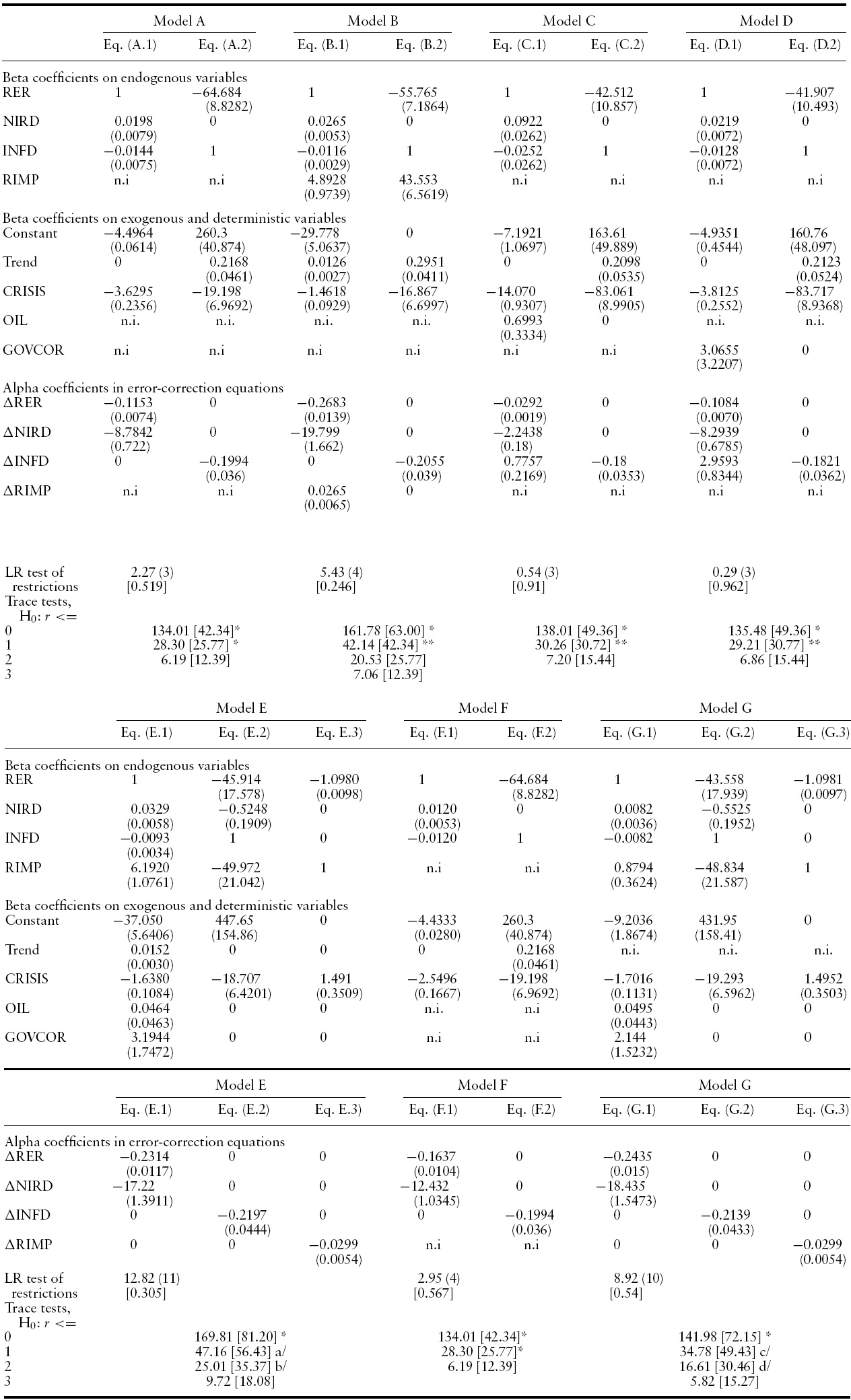
Table 4 presents the estimation results for a sequence of models. Model A starts with the real exchange rate and the interest and inflation differentials as endogenous variables; and a constant, linear trend, and CRISIS dummy as deterministic components. The sequence adds the manufacturing production ratio (model B), the oil price (model C), government consumption (model D), and finally all the variables together (model E). Models F and G, also included in the table, will be explained below.
In all the models, the trace test indicates the existence of two cointegration relationships, which after the imposition of identifying restrictions – amply accepted by the LR test – can be interpreted as long-run equations for the inflation differential and the real exchange rate. The critical values for the trace test were taken from Pesaran
In the different models the negative and highly significant alpha coefficients indicate that the inflation differential and the real exchange rate adjust over time toward their long-run levels as determined by the cointegration equations. In models E and G, the alpha coefficient in the error-correction equation for the manufacturing production ratio indicates a statistically significant but very slow adjustment of that variable toward its long-run level. The slow adjustment probably reflects the fact that – through the choice of variables – the models were set up to study the equilibrium in the assets market rather than the determination of the production level. Ibarra (2008c) shows, for instance, that an acceptable model for industrial production in Mexico must include investment and manufactured exports, besides the real exchange rate.
[Table 3.] VAR diagnostics 1990Q1-2006Q4, 68 observations
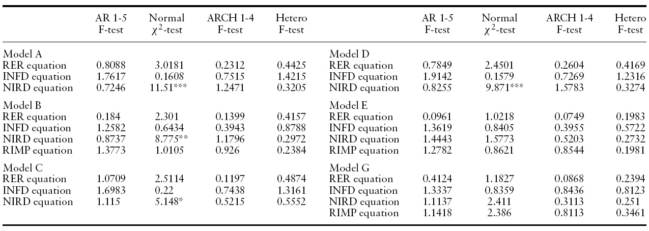
VAR diagnostics 1990Q1-2006Q4, 68 observations
[Table 4.] BEER models Johansen’s ML estimation, 1990Q1-2006Q4, 68 observations
BEER models Johansen’s ML estimation, 1990Q1-2006Q4, 68 observations
In the cointegration equations for the inflation differential and the manufacturing production ratio, the real exchange rate is the most significant determinant. The real exchange rate has a positive effect on the production ratio, with an elasticity practically equal to one (Ibarra, 2008c provides evidence that the channels for this effect are investment and manufactured exports). The real exchange rate also has a positive effect on the inflation differential.11 The estimated coefficient implies that a 10% appreciation tends to decrease the inflation differential in about 6.4 to 4.2 percentage points (see equations A.2 and D.2).
Considering now the cointegration equation for the real exchange rate, the coefficients on the three real-side determinants show the expected negative sign. Only the manufacturing production ratio, though, is always statistically and economically significant; moreover, its inclusion improves the overall estimation results: both the interest-differential coefficient in the real-exchange-rate cointegration equation and the speed of adjustment of the real exchange rate toward its long-run level rise (compare models B and E, with model A).
The negative coefficient on the manufacturing production ratio presumably reflects the Balassa–Samuelson effect. Figure 1 shows that the rise in the production ratio contributed to the real appreciation of the peso during 1990–1991 and again in the second half of the 1990s. The estimated coefficient in equation E.1, for instance, implies that the rise in the production ratio explains about 7.7 points (0.0124 times 6.192) of the 19% appreciation recorded during 1998–2001. Note, however, that the manufacturing production ratio – since it was falling – cannot explain the strong appreciation observed during 1992–1993.
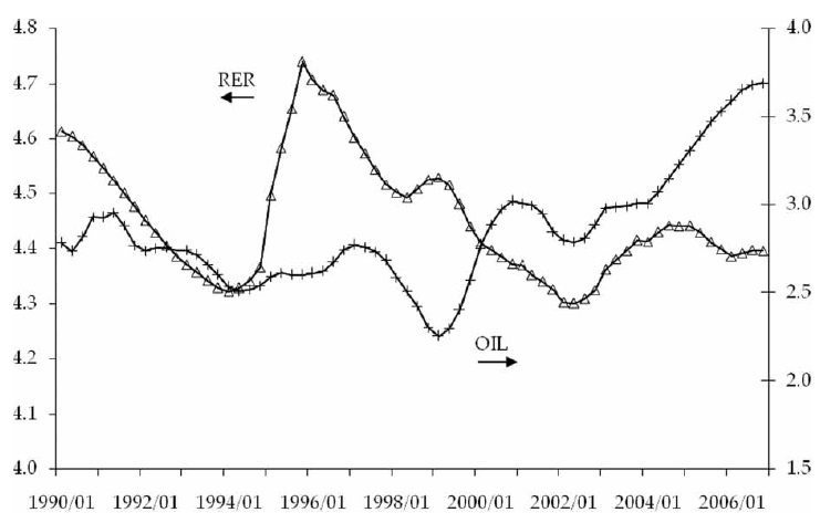
There is some evidence of an oil-price effect on the real exchange rate. The negative coefficient in equations C.1 and E.1 implies that the oil price may have contributed to the peso appreciation during 1999–2000 and 2004–2006. The appreciation registered in the 1990s, though, is necessarily unrelated to the evolution of oil, which mostly tended to fall (see Figure 2). In addition, equation C.1 – the only one where the oil price is statistically and economically significant – is not entirely satisfactory: the speed of adjustment of the real exchange rate drops from 0.2683 in equation B.1 to 0.0292, and the CRISIS coefficient turns unrealistically large. The lack of a robust effect of the oil price on the peso’s real exchange rate may reflect the decline of this commodity in Mexico’s international trade.12
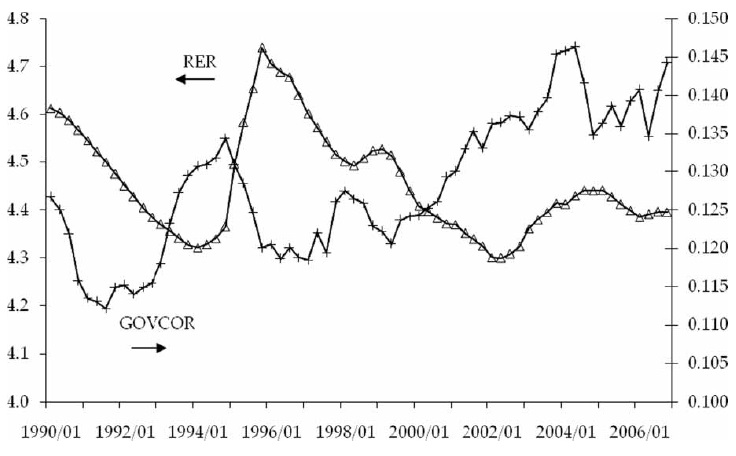
The negative coefficient on government consumption suggests that this variable contributed to the peso appreciation during 1992–1993 and 1998–2001 (see Figure 3), but the effect is probably small.The coefficient in equation E.1 – the one where it approaches statistical significance – implies that the rise in government consumption during 1998–2001 tended to appreciate the peso by about 1.4% (3.1944 times 0.007) – against a total appreciation of 19%.
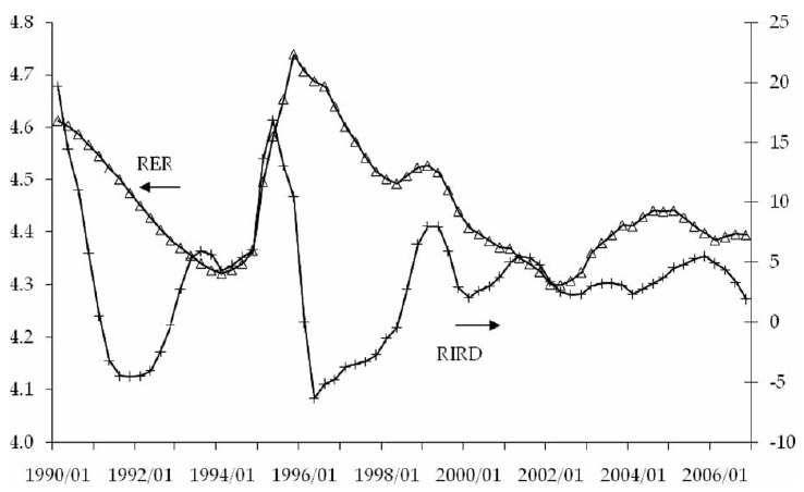
Figure 4 reveals a complex relationship between the real interest differential and the real exchange rate. At times of financial turbulence – like 1994–1995 (the Tequila crisis) and 1998–1999 (the Russian crisis) – the variables move in the same direction, probably reflecting the policy use of the interest rate to cushion the impact on the exchange rate. Over prolonged periods, though, they tend to move in opposite directions. For instance, the appreciation of the peso during the early 1990s, and again in the wake of the 1995 crisis, took place against the backdrop of a rising interest differential.
The link is captured in the estimated long-run equations for the real exchange rate, which show a positive relationship of that variable with the inflation differential and a negative one with the nominal interest differential. The result obtains whether the real-side variables are excluded (model A), included one by one (models B to D), or simultaneously (model E).
Finding a negative relationship between the exchange rate and the interest rate is important, for it implies that causality runs from the interest rate to the exchange rate, thus validating the risk-adjusted parity condition underlying the BEER model. As mentioned in section 3, a positive relationship would signal that the interest differential is in fact being determined by the exchange rate – a policy of leaning against the wind.
Taken together, the equations for the inflation differential and the real exchange rate imply that the nominal interest differential has a long-run effect on the real exchange rate by two channels: directly, through a rise in the real interest differential; and indirectly, through a fall in the inflation differential.
To exemplify, consider model A. The direct channel, captured by the real exchange rate equation (A.1), shows that a rise of 5 points in the interest differential eventually leads to a real currency appreciation of 10% (5 × 0.0198). The indirect channel operates through inflation: a 10% real currency appreciation decreases the inflation differential by 6.5 points (0.1 × 64.684; see equation A.2), which in turn tends to produce a further 9% appreciation (6.5 × 0.0144). Naturally, the specific numbers must be taken with caution, but they do suggest that variations in the interest differential can have economically significant effects on the real exchange rate.13
To have an idea of the historical effects in the Mexican case, consider that the real interest differential rose by 7.5 percentage points during 1998–2001, resulting from a fall of 14.9 points in the inflation differential but of only 7.4 points in the nominal interest differential. According to the estimated coefficients in equation A.1, this tended to produce a real appreciation of 6.8% – that is, about one third of the appreciation recorded in that period.
Note, however, that using the coefficients of equation E.1 – instead of A.1 – would predict a
Two models were estimated under the symmetry restriction: model F, which excludes the real-side determinants of the real exchange rate (originally, model A), and model G, which includes all the variables (originally, model E). The new models are accepted by the LR test with
The estimated coefficients in the new models have the expected sign, indicating that a rise in the real interest rate differential – irrespective of whether it comes from a rise in the nominal interest rate or a fall in the inflation differential – tends to produce a lasting currency appreciation. The point estimate of 0.0082 – to use the smallest of those obtained in models F and G – implies that the observed rise of 7.5 points in the real interest differential during 1998–2001 tended to produce a real appreciation of 6.2% – representing, again, about one-third of the actual appreciation recorded in the period.
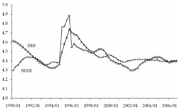
As a summary of the different effects, Figure 5 shows the actual real exchange rate together with the estimated BEER series from model G. The figure suggests that, after controlling for the influence of real-side and monetary factors, the peso was overvalued in about 9% by 2002. This is in addition to the already mentioned effect of the rise in the real interest differential. Understanding the strong appreciation of the peso in the late 1990s and early 2000s is clearly a topic for further research.
9An F-test showed that no lag could be eliminated; in addition, removing the fourth lag introduced serial correlation in the residuals. 10The trace statistic was corrected for small-sample bias using the factor suggested by Johansen (2002) (see note inTable 4). Following standard practice, the cointegration relationships are reported in the form β´x = 0. The estimations were carried out in PcGive 10. 11In most models the interest differential in the inflation equation has a non-significant coefficient. If in equation E.2 the interest differential –which shows a significant positive coefficient – is eliminated, then the real exchange rate coefficient rises strongly, from45.9 to 88.3; this suggests that the positive coefficient on the interest differential is capturing some of the inflationary effect of the real exchange rate during periods of financial turbulence – when the interest differential and the real exchange rate move in the same direction. Eliminating the interest differential, however, is rejected at 10% by the LR test. In the inflation equation of models E and G, the manufacturing production ratio has a positive coefficient, presumably reflecting a cost-push factor. 12The share of oil in goods exports fell from more than 60% in the early 1980s to less than 10% twenty years later. The variable has been problematic in previous studies. Kildegaard (2006) found a significant but positively-signed oil price coefficient in a cointegration analysis for the period 1969–2000; Dabós and Juan-Ramón (2000) obtained a similar result in a regression analysis for the period 1982Q1–1998Q4 – using the international terms of trade rather than the oil price. Edwards (1994) and Elbadawi (1994) discuss theoretically why the terms of trade coefficient may have an ambiguous sign. 13Interestingly, our point estimates for the interest-differential coefficient in the long-run equation for the real exchange rate are very similar to those obtained by Frankel (2007) in his study of the South African rand (his point estimates range from0.019 to 0.022 for the pre-liberalization period). 14A larger coefficient on the inflation differential was expected under the assumption that the inflation differential could be a significant determinant of the unobserved risk premium. Following the BEER literature, model A was re-estimated with the addition of the government’s total debt (in percentage of GDP) as a possible determinant of the risk premium (results available upon request). As expected – given the stationarity of the new variable – the trace test indicated the existence of a new, third cointegration relationship, which captured a positive relationship between government debt and the interest differential. The estimated coefficient on the government’s debt in the longrun equation for the real exchange rate showed the expected positive sign, but no economic or statistical significance. Compared with model A, the other coefficients in the real exchange rate equation remained unchanged, including those on the interest and the inflation differentials. 15The trend had to be removed from model G for the LR test to accept the symmetry restriction.
In a setting of prolonged disinflation, since the late 1980s theMexican peso experienced a tendency to appreciate in real terms. Controlling for the effect of real-side variables, such as relative manufacturing production, government consumption, and the oil price, the paper showed that monetary policy – as reflected in the interest differential – had a lasting effect on the peso’s real exchange rate.
A frequent assumption in the academic literature and the policy debate is that monetary factors – in contrast to real-side determinants – cannot have a lasting effect on the real exchange rate. The premise does not seem suitable in Mexico’s case, however, given the country’s experience of prolonged disinflation and the sustained focus of monetary policy on that goal.
To test the joint influence of real-side and monetary variables, the paper estimated a BEER (Behavioral Equilibrium Exchange Rate) model for the Mexican peso. The model not only considers both types of variables, but relies on Johansen’s cointegration methodology – a natural framework to uncover longrun effects on the real exchange rate. The period under analysis starts in 1990Q1 (to concentrate on the period of free capital mobility in Mexico, as required by the risk-adjusted interest parity condition underlying the BEER model) and ends in 2006Q4.
In different combinations, the core of the estimated models consisted of the real exchange rate – the inverted consumer-price ratio between Mexico and the US – and the nominal interest differential, the inflation differential, and the manufacturing production ratio between the two countries, all as endogenous variables; and the international price of oil in real terms and Mexico’s ratio of government consumption to GDP as exogenous variables.
Johansen’s methodology yielded models of two cointegration relationships that can be interpreted as long-run equations for the real exchange rate and the inflation differential; in some models the estimation produced an additional equation, for the manufacturing production ratio. The models show that the manufacturing production ratio and the inflation differential depend positively on the real exchange rate, while the real exchange rate – controlling for the effect of real-side variables – depends negatively on the nominal interest rate differential and positively on the inflation differential. Taken together, the equations for the inflation differential and the real exchange rate imply that a rise in the nominal interest differential appreciates the currency by two channels: directly, through a rise in the real interest differential; and indirectly, through a fall in the inflation differential.
The effect of the interest differential on the real exchange rate is economically significant. Using the estimated coefficients in the cointegration equation for the real exchange rate shows, for instance, that the 7.5 point rise in the real interest differential recorded during 1998–2001 accounts for about one-third of the real appreciation observed in the period.