There is a large literature suggesting a robust positive relationship between financial development and economic growth. This view dates back to Schumpeter (1911) who argued that the banking sector plays a key role in economic development, by choosing which firms have the best chance to succeed in the innovation process. The works of Gurley and Shaw (1955), Goldsmith (1969), McKinnon (1973) and Shaw (1973) subscribe to this line. During the last 25 years, by the use of various methodologies, several empirical studies have shown that financial development is not only positively linked to economic growth, but also a good predictor of economic development. Moreover, by increasing intermediation, financial development encourages savings and investment and improves the allocation of savings to investment projects. This in turn leads to high level and great efficiency of capital, which finally stimulates economic growth.1 Although the favourable effect of financial development on growth, only a fewstudies asked whether there are certain conditions that can be associated with a stronger or weaker relationship between the two variables. In this paper, we examine the way in which the finance–growth relationship can vary according to the inflation rate. The variation of this relationship with the inflation rate suggests the existence of non-linearity between both variables and questions the hypothesis made in cross-section and traditional panel data regressions.2 The non-linearity between finance and growth with respect to inflation might be connected to the fact that inflation negatively affects economic growth and thus results in financial repression.
First, several studies report the negative influence of inflation on growth.3 The effects of inflation on the real sector can be either direct or indirect. Inflation increases transactions and information costs, and then impedes efficient resource allocation by obscuring the signals resulting from price changes. In such an environment, characterized by imperfection of the information about prices, economic agents will be reluctant to enter contracts; this penalizes investment and inhibits economic growth. To support this view, Sarel (1996) shows that a structural break exists in the relationship between inflation and growth. According to the author, an inflation rate higher than 8% exerts a powerful negative impact on growth, while for a rate below 8% the impact of inflation tends to be slightly positive. Inflation could be seen as characteristic of underdeveloped economies. Khan and Senhadji (2001) and Khan (2002) also find that the threshold rate of inflation is around 1–3% for industrial countries, while this value ranges between 7 and 11% for developing countries.4 More recently, by using Panel Smooth Threshold Regression (PSTR) on six industrialized countries, Omay and Kan (2010) find that there exists a statistically significant negative relationship between inflation and growth for the inflation rates above the critical threshold level of 2.52%.
Secondly, the financial sector can be hurt by a high level of inflation rate, which can be a consequence or a result of financial repression.5 Indeed, as previously evoked, in an inflationary environment, financial intermediaries dislike long-term financing, which supports growth because of the greater stock return variability and tends to maintain liquid portfolios. Financial intermediaries also dislike higher volatility of inflation rate, because it would make inflation rate less predictable and increase economic uncertainty. In economies with high inflation, intermediaries will lend less and allocate capital less effectively, and equity markets will be smaller and less liquid. Therefore, higher rates of inflation are associated with lower long-run real rates of return on a broad class of assets, and imply more severe rationing of credit, then reducing financial depth. The banking systems hold a significant quantity of non-interest bearing cash reserves in every economy. As is well-understood, higher rates of inflation act like a tax on real balances or bank reserves. And, if this tax is borne, at least in part, by bank depositors, higher inflationmust lead to lower real returns on bank deposits. Since bank deposits compete with a variety of assets, it is plausible that reduced real returns on bank deposits will result in reduced real returns on a variety of assets (Khan, 2002). High price level also encourages the government to implement financial repression policies6 in order to mobilize resources for public spending and to protect certain sectors of the economy. This situation leads to resources misallocation and has harmful effects on economic growth. Furthermore, by increasing the opportunity costs of holding money, inflation causes a lessening of the ratios of money or financial assets to GDP. Khan
In spite of the usefulness of the analyses of the relationship between growth and inflation on one side and finance and inflation on the other side, these studies do not allow us to directly conclude with respect to the impact of financial development on the inflation–growth nexus or the impact of inflation on the finance–growth link. Therefore, only a few studies appraise the relationship between inflation, financial development and growth. Rousseau and Wachtel (2002) point out the existence of threshold effects in the finance–growth nexus, by considering the inflation rate for a sample of 84 countries between 1960 and 1995. Their results suggest that the inflation threshold of the finance–growth relationship lies between 13 and 25%.When the inflation rate exceeds the threshold, finance ceases to increase economic growth. More recently, Rousseau and Yilmazkuday (2009) have extended the work of Rousseau and Wachtel (2002) through a trilateral graphic approach and threshold analysis. They find that small increases in the price level seem able to wipe out relatively large effects of financial deepening when the inflation rate lies between 4 and 19%, whereas the finance–growth relationship is less affected by inflation rates above this range. Huang
Results suggesting a non-linear relationship between inflation, finance and growth were also obtained by Gillman and Harris (2004) from simple regressions of the growth-containing interaction variable, which is the product of inflation and financial depth. Nevertheless, Haslag and Koo (1999) find that inflation is never significant in growth regressions that include financial development. Indeed, the results obtained by these authors are surprising as far as the coefficient of the interaction variable (the product between inflation and financial development) is positive.
The main limit of all previous studies consists of assuming that, the relationship between finance and growth can only be affected by cross-country variation of the inflation level, and neglecting inflation change over time. This study fills this gap through the use of Panel Smooth Threshold Regression (PSTR).7
According to Gillman and Harris (2004), and Khan (1999), the channel through which inflation affects growth may run, at least in part, through the financial sector. The topic of this paper is to analyze how the finance-growth nexus is affected by the inflation rate. To do this,we use the methodology of Panel Smooth Threshold Regression (PSTR) developed by Gonzàlez
Our results suggest that the relationship between financial development and economic growth is non-linear and this link can be affected by the inflation rate. At the same time, there is an inflation threshold for the finance–growth nexus. Furthermore, we show that an increase in the price level negatively affects growth through financial developmentwhen the inflation rate is higher than 20%,whereas the impact of finance on growth is positive and significant for an inflation level below 10%.When inflation lies between these two thresholds the finance–growth relationship is positive but very weak.
The rest of the paper is organized as follows. In the next section, we discuss the threshold specification regression. The third part of the paper resumes the main results obtained from the panel threshold estimations. The last section concludes.
1See King and Levine (1993), Beck et al. (2000), Levine et al. (2000), Demetriades and Hussein (1996) and Rousseau and Wachtel (1998) for empirical assessments of the finance–growth relationship. Levine (1997, 2005) also provide a useful survey on the subject. 2The traditional regressions suppose that the finance–growth relationship is linear; it implies that the finance–growth coefficient is constant in time and across countries. 3See Fischer (1993), Barro (1996), Bruno and Easterly (1998) and Hung (2003). Temple (2000) also discusses why inflation should be related to growth and surveys the empirical literature. 4However, using a data set of OECD countries, Andrés et al. (2004) show that, if inflation affects growth through its interaction with financial market conditions, this is not the only channel. They also find that the long-run costs of inflation are not explained by policy of financial repression. 5Although the correlation between inflation and financial repression is established, notice that the causality between both variables remains little documented and can be extended in further studies. 6Financial repression policies can occur by a ceiling interest rate, or by obliging banks to finance governmental projects. 7Notice that inflation is not the only source of non-linearity between finance and growth. This nonlinear relationship can also depend on structural parameters as well as on variables of economic policies. For more details see Berthélemy and Varoudakis (1995, 1996), Aghion et al. (2005), Deidda and Fattouh (2002, 2008), Gaytan and Rancière (2004), Ketteni et al. (2007), and Huang and Lin (2009).
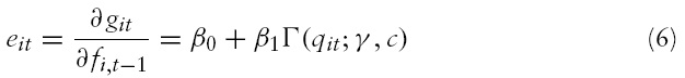
The basis of our model is exactly the same as the one used by many authors who investigate the finance–growth relationship on panel data. The corresponding equation is then defined as follows:

where

This model, which is used for the first empirical estimations of the finance–growth relationship, presents two main drawbacks. First, it supposes that the finance-growth coefficient remains for all the countries of the sample. Second, this model implies that the finance-growth coefficient is constant in time. It seems unrealistic as the effect of financial development on growth at the beginning of the 1960s might be different from its effect in the 2000s. To solve these problems, we can suppose that the panel is heterogeneous and consequently parameter (
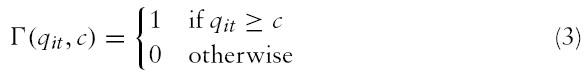
One solution to circumvent both these issues consists of introducing threshold effects in a linear panel model. In this context, the first solution requires using the Panel Threshold Regression (PTR) model (Hansen, 1999) as suggested by Deidda and Fattouh (2002). In this case, the mechanism of transition proposed by Hansen (1999) between extreme regimes is very simple: at each date, if for a given country, the transition variable is lower than a given value, called the threshold parameter (which is in our case the inflation rate), then the finance–growth model is defined by a particular regime, and this regime is different from the model used if the transition variable is larger than the threshold parameter. For instance, let us consider a PTR model with two extreme regimes:

where

with such a model, the finance-growth coefficient is equal to (
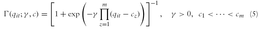
The conventional solution to this problem is the use of a model with a smooth transition function. This type of model, commonly used in time series analysis, has recently been extended to panel data with the Panel SmoothThresholdRegression (PSTR) model proposed by Gonzàlez

The transition function Γ is continuous and depends on the threshold variable

The main advantage of PSTR is that it allows the finance-growth coefficient to vary according to the country and in the time dimension; hence it provides a parametric approach of cross-country heterogeneity and of time instability of the finance-growth coefficients, since these parameters change smoothly as a function of a threshold variable,which in our case is the inflation rate. The finance–growth coefficient for the
According to the properties of the transition function, we have
Another advantage of the PSTR model is that the finance–growth coefficient may be different from the estimated parameters for extreme regimes, i.e.
Although these expressions of the elasticity allow some configurations for the finance and growth relationship, several questions relative to estimation and specification tests persist. The next section is devoted to answering them.10
>
Estimation and Linearity Test
The PSTR model estimation consists of several stages. It begins by removing individual-specific means and then by applying non-linear least squares to the transformed model.11 Then, we use the following testing procedure: first, the linear against the PSTR model is tested,12 and, second, the number

Since

where
Once the linearity test is used, the problem is to identify the number of transition functions in the model.The sequential approach by testing the null hypothesis of no remaining non-linearity is generally used. If the linearity hypothesis has been rejected, the issue is then to test whether there is one transition function (

Γ1(

The test of no remaining non-linearity is simply defined by:
Then, the testing procedure is as follows. Given a PSTR with
8We use the lag of the financial development variable to treat the endogeneity problem between financial development and economic growth. 9See next section (data and threshold results) for more details. 10For the analysis of the asymptotic behaviour of the PSTR estimator, see González et al. (2005) and Fok et al. (2005). 11See Gonzàlez et al. (2005) and Colletaz and Hurlin (2006) for more details. 12We assume in our specification that the transition functions have one threshold. If some models require transition functions with more than one threshold, we may use in these cases several functions with one threshold.
This study is based on a selection of 71 developed and developing countries,13 over the period 1960–2004. Our data are taken from PennWorld Tables (PWT 6.2) and from the financial database realized by Beck
[Table 1.] Properties of the data: descriptive statistics, cross-section 1960?2004
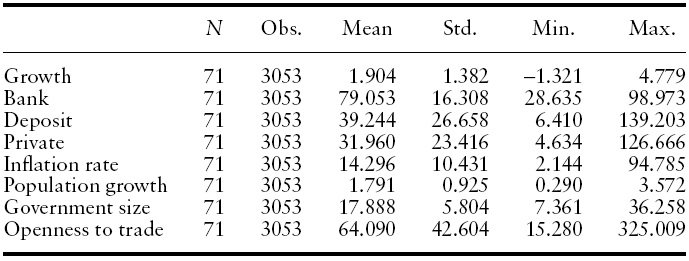
Properties of the data: descriptive statistics, cross-section 1960?2004
We consider three different models (Model A, B and C) according to the financial development indicator. For each model, the first step is to test the linear specification of economic growth versus a specification with threshold effects. If the linearity hypothesis is rejected, the second step will be to determine the number of transition functions required to capture the non-linearity. We make the assumption that in our PSTR model, a single location parameter is used in the logistic transition function (i.e.
[Table 2.] LMF tests for remaining non-linearity

LMF tests for remaining non-linearity
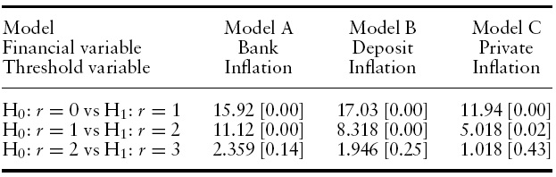
The results of these linearity tests are reported in Table 2. For each model (indicator of financial development), we compute the statistics for the linearity tests
The specification tests of remaining non-linearity led also to the identification of the optimal number of transition functions or extreme regimes. As reported in Table 2, for all three tests, the null hypothesis of the remaining non-linearity cannot be rejected for
[Table 3.] Parameter estimates for the final PSTR models

Parameter estimates for the final PSTR models
The specification of the estimated equation for the final PSTR model is the following:16

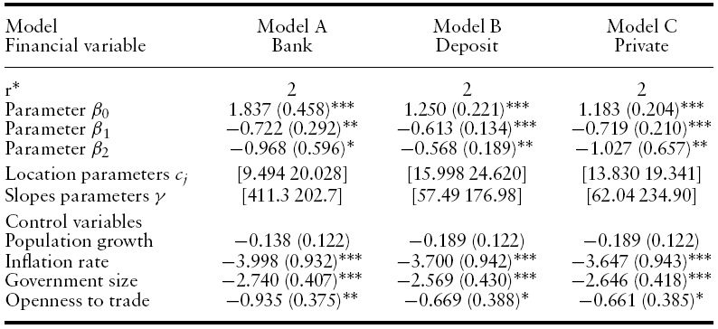
Table 3 contains the parameter estimates of the final PSTR model (with two transition functions). The control variables have the expected signs: the inflation rate, the ratio of government expenditure to GDP and the openness to trade have a significant negative impact on economic growth,while the effect of the population rate is not significant.
We note that the estimated values of the slope parameters
As mentioned above, the estimated parameters
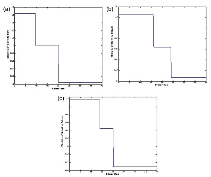
Then, our results suggest that for the low level of inflation rate the financegrowth coefficient lies between 1.183 and 1.837. For an inflation rate lying between 9.494% and 24.620%, the finance-growth coefficient is 1.115, 0.637 and 0.464 for BANK, DEPOSIT and PRIVATE, respectively. By contrast, for a high level of inflation (i.e. higher than the last threshold), the sensitivity of growth to finance is 0.147, 0.068 and −0.563 respectively for BANK, DEPOSIT and PRIVATE.17 The decline of the finance–growth coefficient shows that a macroeconomic environment characterized by a high level of inflation is less convenient for a favourable impact of financial development on growth.
For a better illustration of the impact of the inflation level on the finance–growth relationship, Figure 1 depicts the elasticity defined by equation (6) against the inflation rate, and derives three balances for all models. Furthermore, Model A shows that for an inflation level less than 9%, the finance–growth coefficient is close to 1.84; this value is near1%for an inflation rate between 9 and 20%. Indeed, beyond an inflation threshold of 20%, economic growth is no longer sensitive to financial development. The same conclusion can be drawn fromthe other models with a slight change in the thresholds and the finance–growth coefficients. This suggests the robustness of our results to various financial development indicators.
Our results are similar to those obtained by Rousseau and Wachtel (2002). However, our results allow for more debate assessment of the implications of the inflation on the finance–growth relationship: three equilibria are identified according to inflation rate; that is not the case in Rousseau and Wachtel’s paper.
Overall, the estimation of the non-linear relationship between finance and growth with respect to the inflation rate highlights that, in countries that record high inflation, economic growth is less sensitive to financial development. Therefore, an economic policy that aims to increase the sensibility of growth to finance will control and fight inflation.
13The sample is the following: 18 low-income countries (Burkina Faso, Burundi, Ivory Coast, Ethiopia, Gambia, Ghana, Haiti, India, Kenya, Madagascar, Nepal, Niger, Nigeria, Pakistan, Rwanda, Senegal, Sierra Leone, Togo); 30 middle-income countries (South Africa, Argentina, Barbados, Bolivia, Chile, Colombia, Costa Rica, Egypt, El Salvador, Ecuador, Gabon, Guatemala, Honduras, Iran, Jamaica, Malaysia, Morocco, Mauritius, Panama, Dominican Republic, Paraguay, Peru, Philippines, Seychelles, Sri Lanka, Syria,Thailand,Trinidad andTobago, Uruguay,Venezuela); 23 high-income countries (Australia,Austria, Belgium, Canada, Cyprus, Denmark, Finland, France, the UK, Greece, Iceland, Ireland, Israel, Italy, Japan, Norway, New Zealand, the Netherlands, Portugal, Singapore, Sweden, Switzerland, the USA). The countries are selected according to the data availability. 14Financial development is measured only through banking sector indicators. We don’t use in this paper stock market indices, given that these variables are only available for developed countries. 15However, in the case of a model with at most one threshold for each transition function, Colletaz and Hurlin (2006) suggest the use of the testing procedure proposed by Granger and Teräsvirta (1993) which can be adapted in the case of PSTR models so as to choose between m = 1 and m = 2. Except for this special case, there is no general specification test for the choice of m. 16A positive correlation between financial development and growth variables in this paper means that financial development has a positive effect on economic growth. I would like to thank the referee for this suggestion. 17These values are derived from the derivation of the PSTR growth equation (equation (11)) and are highlighted in Figure 1.
Conclusion and Policy Implications
The recent empirical literature has shown that the relationship between financial development and economic growth is mostly positive, and significant. However, the impact of the inflation rate on this link is not often questioned in the literature. This paper helps to shed light on the complex interaction between financial development, inflation rate and economic growth, using the methodology of Panel Smooth Threshold Regression (PSTR) developed by Gonzàlez
Our results highlight serious macroeconomic consequences of not avoiding excessive inflation on economic growth. These results provide strong empirical confirmations of the economic policy, which recommends low inflation for a strong relationship between the financial and real sectors.The policy implications derived from these findings consist of the development of institutional arrangements for controlling and fighting inflation, for maintaining macroeconomic stability, and for encouraging the real impact of financial policy on economic growth.