In the world that existed before the global financial crisis, interest rate rules, especially the Taylor rule, dominated the debate and research on monetary policy. During the financial crisis, however, the consequences of an increase in the money supply have returned the monetary policy debate due to the two rounds of quantitative easing implemented by the US Federal Reserve. An important question about this monetary policy is not only its ability to stimulate the economy, but also its impact on the external value of the dollar.
Since the collapse of the post-war BrettonWoods system of fixed exchange rates in 1973, the era of floating currencies has been associated with large exchange rate fluctuations. The determination of floating exchange rates has been one of the main areas of research in international economics. Reasons for the high volatility of exchange rates have attracted much attention.
Two broad classes of theories have been developed to explain large exchange rate fluctuations. Since the publication of the ‘overshooting model’ by Dornbusch (1976), one strand of the exchange rate literature has developed sticky price monetary models, which could account for large fluctuations in exchange rates that would be consistent with the rational expectations hypothesis.1 An alternative and popular view is that the main cause for large exchange rate fluctuations is destabilising speculation (see for example Krugman, 2002).
One of the most important determinants of the nominal exchange rate is the relative money supply. In the traditional monetary approach to the exchange rate, the classical exercise to carry out is to analyse the effects of an unexpected permanent increase in the money supply. In the overshooting models of Betts and Devereux (2001), Dornbusch (1976) and Obstfeld and Rogoff (1996, Appendix), an increase in the money supply induces an immediate jump in the nominal exchange rate,which is followed by a gradualmovement over time to the newlevel. As emphasised, for example by Dornbusch and Frankel (1995) and by Frydman and Goldberg (2007), the overshooting model(s) cannot explain why exchange rates also tend to undergo gradual swings away from benchmark levels.
Empirical literature provides mixed evidence on the exchange rate overshooting hypothesis. As emphasised by Bjørnland (2009), empirical studies of monetary policy have typically found exchange rate effects that are inconsistent with overshooting. Instead, they have found support for the view that the response of the exchange rate is only gradual.Thus, that in the short run, the exchange rate undershoots its long run value. Bjørnland (2009), on the other hand, finds support for the overshooting hypothesis.
Papell (1984) shows that accommodative monetary policy can switch from exchange rate overshooting to undershooting.He develops a two-country version of the Dornbusch model, in which the domestic and foreign money supply are endogenously determined. The central banks in both countries follow simple money supply rules, so that the money supply depends on both the exchange rate and the difference between domestic and foreign prices. In his framework, a monetary policy that tries to offset exchange rate movements and accommodates price movements can be interpreted as an attempt to stabilise output. The author shows that an active monetary policy that accommodates price movements can cause exchange rate undershooting.
The purpose of this study is to examine whether the undershooting result of Papell (1984) is valid in an optimising framework. To address this question, the standard New Open Economy Macroeconomics (NOEM)2 model is extended with the introduction of a hypothetical money supply rule that captures the main idea of the Taylor rule (Taylor, 1993). The monetary policy rule proposed here assumes that central banks in both countries change the money supply if the actual level of output diverges from the potential level of output, or if the actual rate of inflation diverges from the target rate of inflation.
The main result of this paper is that Papell’s (1984) conclusion that money supply rules can cause exchange rate undershooting is valid in an optimising framework. If the level of technology improves, or if a country faces a monetary shock, then the nominal exchange rate does not follow a random walk. If the exchange rate models of Betts and Devereux (2000), Dornbusch (1976) and Obstfeld and Rogoff (1996, Appendix) can account for a long swing towards the new long-run level, the present model provides an explanation of a long swing away from the benchmark level.
The rest of this paper is organised as follows. Section 2 presents the model. Section 3 discusses the implications of monetary policy rules for exchange rate dynamics. Finally, section 4 concludes.
1This literature includes Frenkel (1976), Frankel (1979), Mussa (1979) and Buiter and Miller (1982); more recent contributions include Obstfeld and Rogoff (1995, 1996) and Betts and Devereux (2000). 2Surveys of the NOEM literature are presented by Lane (2001), Lane and Ganelli (2003) and Corsetti (2007).
In this section, I develop a standard two-country NOEM model that is based on Betts and Devereux (2000). They modified the Obstfeld–Rogoff model by assuming that a fraction of firms set their prices in the customer’s currency. However, I focus exclusively on the traditional producer currency pricing (PCP) case, assuming that prices are rigid in the producer’s currency. I extend the Betts–Devereux model in three ways. First, I assume that central banks follow a hypothetical monetary policy rule whereby they change monetary policy if the actual level of output or inflation diverges from their target levels. Second, I introduce a Calvo-type staggered price setting. Third, I introduce shocks to the production function.3
2.1 Country Size and Market Structure
The world consists of two countries, home and foreign. There is a continuum of firms and households that are indexed by
2.2.1 Preferences
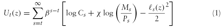
All households have identical preferences. The utility function of the representative domestic household is given by4

Here
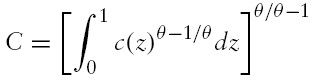
where

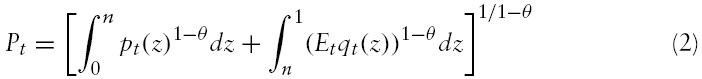
Prices
2.2.2 Budget constraints and first-order conditions
The budget constraint of the representative domestic household is

Here

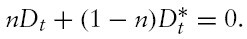
The global asset-market-clearing condition requires
The first-order conditions are


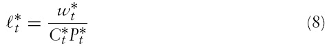

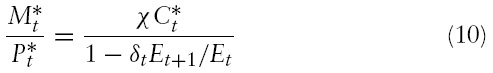
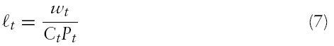
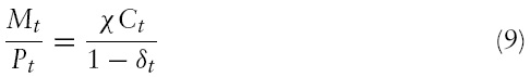
Equations (5) and (6) are the Euler equations for optimal domestic and foreign consumption, respectively. Equations (7) and (8) govern the optimal labour supply, which is an increasing function of the real wage and a decreasing function of consumption. Equations (9) and (10) show that the demand for money is an increasing function of consumption and a decreasing function of the interest rate.
2.3.1 Money supply shocks
The NOEM literature, pioneered by Obstfeld and Rogoff (1995), has often modelled monetary policy in terms of the central bank’s control of the money supply. The standard analysis of monetary policy is to study the international effects of an unexpected permanent increase in the domestic money supply.Asalient feature of NOEM models is that the foreign central bank does not react to the domestic policy expansion. In this basic case, the money supply follows a first-order autoregressive process that can be described by the following equation

where percentage changes from the initial steady state are denoted by hats, and

is an unpredictable shift in the money supply. Shocks to this equation are referred to as money supply shocks.
Since the publication of Obstfeld and Rogoff (2002), a new strand of the literature has analysed monetary policy feedback rules in the face of productivity shocks.6 The object is to find the optimal money supply rules that maximise welfare. This type of analysis could be referred to as ‘normative analysis of monetary policy’. In this study, I do not presume this type of optimisation by central banks; instead I assume that central banks follow a monetary policy that tries to capture the spirit of the Taylor rule (Taylor, 1993). This type of ‘positive analysis of monetary policy’ presents an alternative approach to those of Obstfeld and Rogoff (2002) and related work.
2.3.2 Simple money supply rule
As emphasised byWoodford (2003, Chapter 1), theoretical analyses of monetary policy have, until recently, virtually always modelled monetary policy in terms of a path for the money supply, and discussions of monetary policy rules have mainly considered money growth rules. In more recent analyses of monetary policy, policy is described in terms of rules setting a nominal interest rate.
In this study I make use of a simple money supply rule that tries to capture the spirit of the Taylor rule. The Taylor rule can be written as follows:

Strictly speaking, this rule has the feature that the central bank raises the nominal interest rate (

or if output (

The coefficients
In this study, I consider a monetarist variant of the Taylor rule, similar to the rule used by Pierdzioch (2004). Assume, for the sake of argument, that the domestic central bank follows the following log-linear money supply rule (the foreign central bank follows an identical rule):

In this equation, the coefficients

is the inflation target and

is inflation, and

is an unpredictable shift in the money supply rule. Following new Keynesian closed economy models (see for example Gali 2003), I define the output gap
as the deviation of output from its equilibrium level in the absence of nominal rigidities. Shocks to equation (13) are referred to as shocks to the monetary policy rule.
In NOEM models, however, current account imbalances imply permanent wealth changes that affect the labour supply. Thus, the new equilibrium level of output is not necessarily the same as the old equilibrium level of output, also in the case of monetary shocks. This definition of the output gap is clearly not perfect since the output gap is not exactly zero in the steady state. However, the output gap is virtually zero in the steady state, and consequently the non-zero output gap in the steady state is likely to have a negligible effect on the results. Finally, in the absence of a growth path for the money supply, the inflation target is zero.
The unpredictable shift in the money supply rule – a monetary policy shock – can be caused by a change in the loss function of the central bank. For example, if the loss function changes such that the central bank adopts a more inflationary monetary policy, it can be thought to be a positive shock to the money supply rule. The shock to the money supply rule follows an AR(1) process
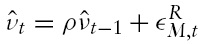
where

is an unpredictable shift in the money supply rule. In the exercise that I carry out in this paper, shocks to the money supply rule are permanent (
Finally, I abstract from government spending so the transfers to households are given by

2.4.1 Technology and profits
Each firm produces a differentiated commodity. The production function of domestic firm

where

where

As mentioned, I use the PCP assumption. The profits of domestic and foreign firms, respectively, are given by


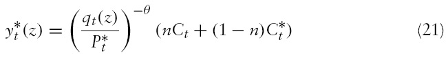
The demands for the products are given by

2.4.2 Price setting
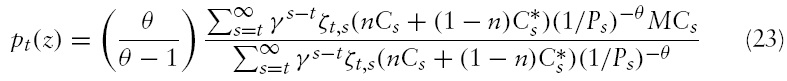
In the absence of nominal rigidities, domestic firms would maximise
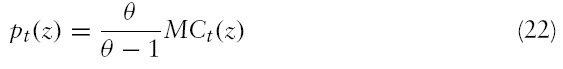
So the price of the commodity would be a constant mark-up over the marginal cost.
In the short run, prices are sticky, and I consider a discrete-time version of the model of Calvo (1983). Each firm resets its prices with a probability 1 −
Domestic firms seek to maximise

where
is the domestic discount factor between period

Foreign firms maximise their profits analogously. The pricing rule for foreign firms is
2.4.3 Symmetric equilibrium
All firms in a country are symmetric, and every firm that changes its prices in any given period chooses the same output and prices. In each period a fraction of firms, 1 −
Equations (14) and (18) can be substituted into equation (3) to derive the consolidated budget constraint of the domestic economy. Making use of the global asset market-clearing condition, the consolidated budget constraint of the foreign economy can be calculated analogously. The consolidated budget constraints can be written as


Following Obstfeld and Rogoff (1995), the model is log-linearised around a symmetric steady state where initial net foreign assets are zero. Equations (7), (15)7 and (22) imply that
where the subscript zero on variables denotes the initial steady state.
The log-linearisation is implemented by expressing the model in terms of percentage deviations from the initial steady state. Those variables whose initial steady state value is zero are normalised by consumption. Equilibrium is sequences of variables that clear the labour, goods and money markets, satisfy the optimality conditions for consumption, satisfy the pricing rules and satisfy the consolidated budget constraints.
3Because the model extends the basic framework, the differences in the results could be coming partly from the monetary policy rule and partly from the staggered pricing mechanism itself. However, as shown in Tervala (2010) and in section 3.3, the Calvo-pricing mechanism does not change the main predictions of the Betts and Devereux (2000) model. 4The equations for the foreign country are identical to those of the domestic country, unless they are explicitly discussed. 5The foreign consumer price index is 6This literature includes Bachetta and van Wincoop (2000), Benigno and Benigno (2003), Corsetti and Pesenti (2005), Devereux and Engel (2003) and Sutherland (2004). 7The initial level of technology is normalised to unity.
3. Money Supply Rules and the Nominal Exchange Rate
The parameterisation of the model is the following. Periods are interpreted as quarters, and thus the discount factor is set to 0.99. The elasticity of substitution between differentiated goods is 6. The Calvo parameter is set to 0.75, which implies an average price duration of four periods. The countries are of equal size, so
In addition, parameter values for
3.2 Shock to the Monetary Policy Rule
I begin by analysing the consequences of shocks to the monetary policy rule. Under perfectly flexible prices, a monetary shock does not affect output

In addition, as mentioned, in the absence of the growth path for the money supply, the inflation target is zero. Thus, the money supply rule can be now written as

I assume a 1% unexpected (permanent) shock
to the money supply rule.
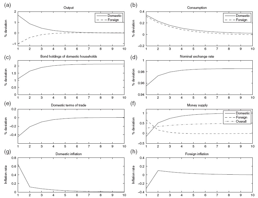
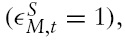
Figure 1 illustrates the dynamic effects of this shock. It is worth observing that the figure shows only the first ten periods and that it takes more than ten periods to reach the new steady state. In the figure, the vertical axes almost always show percentage deviations from the initial equilibrium. The change in bond holdings is, however, expressed as a deviation from the initial consumption, and inflation in period

The domestic terms of trade are defined as the relative price of domestic imports in terms of domestic exports. Thus, the domestic terms of trade deteriorate if this index rises.
Panel (d) in Figure 1 shows that the nominal exchange rate depreciates following a shock to the domestic money supply rule.The log-linear version of equation (10) can be subtracted for the log-linear version of equation (9), and the fact that purchasing power parity (PPP) holds in this model

is used to obtain (the derivation of structural exchange rate equations closely follows the textbook treatment of the Obstfeld–Rogoff model by Walsh, 2003, Chapter 6.2)

where

The log-linear version of equation (6) can be subtracted from equation (5), yielding

This implies that the consumption differential between the countries is constant, as shown in panel (b) of Figure 1. Since PPP holds and the nominal interest rate is equal in both countries, real interest rates are equal across countries. Consumption growth, therefore, is equated across countries, as in the Obstfeld-Rogoff model. In the short run, the liquidity effect of expansive monetary policy decreases the world nominal interest rate, which increases consumption. In addition, the depreciation of the exchange rate improves the foreign terms of trade, increasing foreign consumption in the short run. After the shock, domestic households accumulate net foreign assets. In the long run, higher wealth allows domestic households to keep consumption above output, while foreign households have to decrease consumption to service the external debt.
Making use of equation (30) and the definition of

This equation shows that the equilibrium value of the exchange rate in period
The exchange rate depreciation induces the traditional expenditure switching effect in the short run. This lowers the relative price of domestic goods, causing a shift in world demand towards domestic goods away from foreign goods. This shift in world demand causes a boom in the domestic economy. In addition, the exchange rate depreciation increases the domestic price level, causing inflation. Panel (f) of Figure 1 illustrates that due to inflation and the positive output gap, the domestic central bank tightens monetary policy immediately after the shock, despite the positive shock to the monetary policy rule.When firms have an opportunity to reset their prices, domestic goods become more expensive relative to foreign goods, and the expenditure switching effect peters out. The output gap becomes smaller, and the domestic central bank gradually increases its money supply to the new level consistent with the shock to the money supply rule.
The expenditure switching effect causes deflation and a fall in output in the foreign country in the short run. Deviations of output and inflation from their respective targets force the foreign central bank to implement an expansionary monetary policy. Thus, it expands the money supply in the short run.
Furthermore, panel (d) in Figure 1 also illustrates that, unlike in the Obstfeld–Rogoff model, the nominal exchange rate does not jump immediately to its new long-run level; instead, the exchange rate undershoots its long-run level. The term undershooting (overshooting) refers to the case where the exchange rate changes by less (more) in the short run than it does in the long run when a shock hits the economy. An initial undershooting of the exchange rate is caused by the active monetary policy that both central banks conduct.
Denote

then equation (28) implies that the change in the exchange rate is
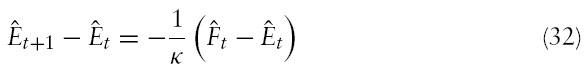
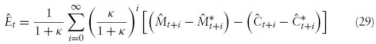
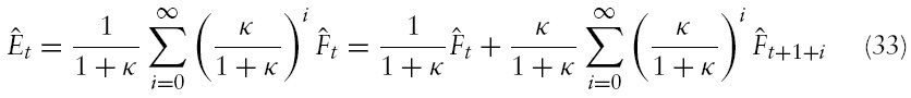
The equation for the exchange rate, equation (29), can be written as

Substituting equation (33) into the right-hand side of equation (32) and using the definition of

implies
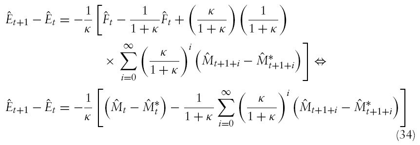
In this equation, the term
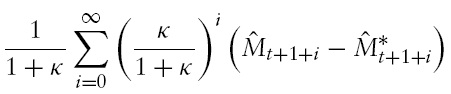
is referred to as the expected future value of the money supply differential. Equation (34) shows the dependence of the change in the exchange rate on the interplay between the current
and expected future values of the money supply differential. For instance, if the current value of the money supply differential is lowrelative to the expected future value of the differential, then the exchange rate must depreciate (see also Walsh, 2003, Chapter 6.2). As mentioned, in the short run, the domestic central bank tightens monetary policy, and the opposite happens abroad. Thus, in the short run,

is temporarily low relative to

and the exchange rate depreciates also after the initial depreciation of the exchange rate. The exchange rate depreciates until the current money supply differential is equal to the expected future value of the differential.
The undershooting result is in contrast with most exchange rate models, but consistent with Papell (1984). He has developed a two-country variable output version of Dornbusch (1976), where the monetary authorities follow a simple money supply rule, which depends on both the exchange rate and the difference between domestic and foreign prices. This rule is quite different from the rule proposed in this paper. However, Papell’s rule implies that monetary policy that accommodates price movements and offsets exchange rate movements can be interpreted as attempting to stabilise output (Papell, 1984).
The findings of this paper generalise the results of Papell (1984): an activist monetary policy can cause exchange rate undershooting. In Papell’s model an increase in the domestic money supply depreciates the steady state exchange rate and increases the domestic to foreign price ratio. The rule implies that this causes the component of the domestic money supply that responds to relative prices to decrease and the foreign money supply to increase. In the terminology of the present model, this implies that there is a difference between the current and the expected future value of the money supply differential. If monetary policy is sufficiently accommodative, the increase in the domestic steady state money supply induces a decrease in the relative (domestic to foreign) money supply. Uncovered interest parity then implies that the domestic interest rate exceeds the foreign interest rate, which is only consistent with expected exchange rate depreciation. Therefore, the exchange rate must undershoot its new long-run level: it must depreciate to a point where it will continue to depreciate.
The effects of monetary shocks on the exchange rate have received considerable attention in the New Open Economy Macroeconomics literature. The standard result in the models based on PPP, such as the Obstfeld–Rogoff model (1995, 1996), is that there is no exchange rate overshooting. However, if PPP is violated by the introduction of non-traded goods (Hau, 2000; Obstfeld & Rogoff 1995, Appendix) or local currency pricing (Betts&Devereux, 2000), then exchange rate undershooting can occur. In these models, the exchange rate undershoots if the consumption elasticity of money demand (1/
As emphasised by Lane (2001), for instance, the intuition is the same as that for the output elasticity of money demand in the Dornbusch model.Ahigh consumption elasticity of money demand means that the domestic interest rate increases relative to the foreign interest rate. Since uncovered interest rate holds, this is possible only if the exchange rate is expected to depreciate. That is, the exchange rate must undershoot its long run value. In this paper, I have shown that accommodative monetary policy can also cause exchange rate undershooting in the model based on PPP, and in the case where the consumption elasticity of money demand is smaller than or equal to one.
Pierdzioch (2005) finds that noise traders, who trade in the foreign exchange market using a simple ‘rule-of-thumb’ when forecasting exchange rates and fail to form rational exchange rate expectations, can cause a delayed overshooting (that is, undershooting in the short run) of the nominal exchange in response to a permanent monetary shock. In this paper, I have shown that accommodative monetary policy can cause exchange rate undershooting in the model with rational exchange rate expectations.
3.3 Money Supply Shock versus a Shock to the Monetary Policy Rule
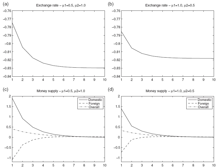
In this section, I compare the effects of a shock to the monetary policy rule with the effects of a simple money supply shock. The dotted lines in Figure 2 show the effects of a shock to the money supply rule, given by equation (27). The solid lines show the effects a money supply shock. That is, a 1% increase in the domestic money supply

governed by equation (11). So the solid lines depict the effects to a monetary shock in the basic Obstfeld–Rogoff (1995) case.
Figure 2 shows that the effects of a shock to the money supply rule are virtually the same as the effects of a simple money supply shock. In panels (a) – (d) it is difficult to see the dashed lines as the effects of these shocks are virtually the same in both cases.The only notable difference between the results is the undershooting of the exchange rate in the casewhere central banks followthe money supply rules. As equations (31) and (34) show, the exchange rate must follow a random walk if the money supply shock is permanent.
The differences in the other results stem from the expenditure switching effect that is driven by the short-run dynamics of the nominal exchange. In the case of a shock to the monetary policy rule, the undershooting of the nominal exchange rate implies a somewhat weaker expenditure switching effect in the short run. Because the response of the nominal exchange rate is quite identical in both cases in the short run, the expenditure switching effect causes only a somewhat smaller increase (decrease) in domestic (foreign) output in the case of a shock to the monetary policy rule than in the case of a money supply shock.
3.4 Technology Shocks and Exchange Rate Dynamics
Since the publication of an influential paper by Kydland and Prescott (1982), the proponents of Real Business Cycle (RBC) theory have supported the view that technological changes are the driving force behind business cycles, at least in developed countries. However, the NOEM literature has mostly focused on exchange rate dynamics caused by monetary or fiscal shocks and the analysis of technology shocks has received much less attention. In addition, a limitation of many NOEM models (including the Obstfeld–Rogoff, 1996, model) is that technology shocks are modelled as shocks to the parameter that captures the disutility of labour. This is more a labour supply shock than a technology shock, as Obstfeld and Rogoff (1996, p. 699) themselves already noted.
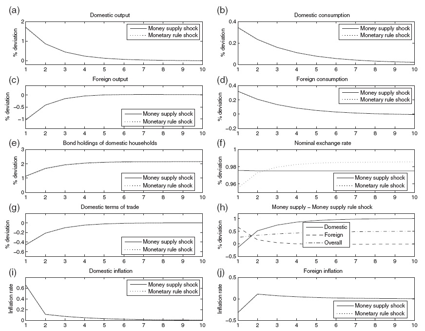
The next step is to examine the consequences of the money supply rules on exchange rate dynamics in the face of technology shocks. Consider a 1% unexpected increase in the level of domestic technology (

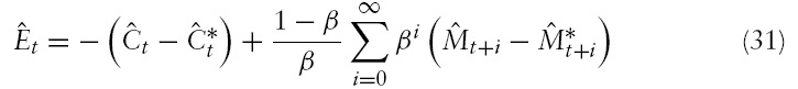
Panel (d) of Figure 3 illustrates that the nominal exchange rate appreciates strongly after a domestic technology shock. A permanent increase in the level of technology leads to a permanently higher level of output. This translates into a higher level of consumption. Equation (31) demonstrates that the relative increase in domestic consumption induces an appreciation of the exchange rate.
The expenditure switching effect of an exchange rate change causes a fall in domestic output and a rise in foreign output in the short run. Domestic goods become more expensive relative to foreign goods in both countries. Consequently, world demand shifts towards foreign goods away from domestic goods. This causes a negative output gap in the home country and a positive one in the foreign country.
A part of the change in monetary policy derives fromthe deviations of inflation from the inflation target. A technology shock decreases the marginal costs of domestic firms, lowering the domestic price level. In addition, the appreciation of the exchange rate decreases the domestic price level (recall equation (2)). A technology shock, therefore, induces deflation in the home country. Deflation and the negative output gap implies that the domestic central bank conducts an expansionary monetary policy until the economy reaches the new steady state. In the foreign country, excess demand allows foreign firms to raise their prices, and, in addition, the appreciation of the exchange rate causes import inflation. The foreign central bank tightens monetary policy to curb excess demand and inflationary pressures.
The undershooting of the exchange rate derives from the monetary policies that the countries implement. As discussed earlier, in the short run, the domestic central bank loosens its monetary policy while the foreign central bank tightens its monetary policy. In terms of equation (34), this means that the current value of the money supply differential is high relative to the expected future value of this differential. Therefore, the exchange rate appreciates also after the initial response. The exchange rate must appreciate until the current money supply differential is equal to the expected future value of the differential.
Adrawback of this analysis is that the output gap is non-zero in the steady state. The reason is that the output gap is defined as the deviation of output from its equilibrium level in the absence of nominal rigidities. In this framework, current account imbalances imply permanentwealth changes that affect the labour supply. Thus, the steady state level of output is not the same as would prevail under perfectly flexible prices. However, the output gap is very small in the steady state, as it is some 0.01%. Thus, the non-zero output gap in the steady state is likely to have only a negligible effect on the results.
As emphasised, for instance, by Lane (2001, p. 261), many results of NOEM models are sensitive to the choice of parameter values. However, the main results of this study are not sensitive to the choice of parameter values. The changes in parameter values do not cause qualitative changes; the consequences on the key results are purely quantitative.
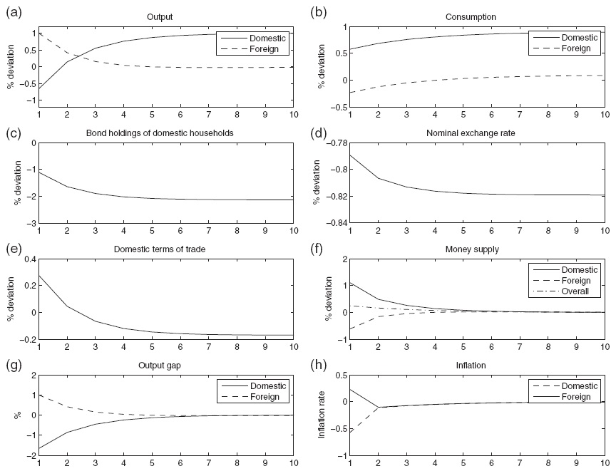
The results of this model can potentially be sensitive to the choice of the coefficients of the monetary policy rule. Thus, I examine the robustness of the findings to changes in these coefficients. Assume, for the sake of argument, that the central banks respond strongly to the deviations of inflation from the target (
Figure 4 shows that if the central banks are more concerned with the output gap than with inflation, then exchange rate fluctuations increase. The intuition behind this result is that if the central banks focus mostly on the output gap, the responses of the central banks are stronger since the deviations of output from their target levels are higher than the deviations of inflation from the inflation targets. Equation (31) demonstrates that the higher the (positive) discounted present value of the money supply differential, the smaller the initial exchange rate appreciation. Equation (34) shows that the higher the current value of the money supply differential relative to the expected future value of the differential, the more the exchange rate appreciates also after the technology shock.
8I simulate the model using the algorithm developed by Klein (2000) and McCallum (2001).
This paper examines the consequences of monetary policy on exchange rate dynamics. In this paper, I propose a simple money supply rule that captures the main idea that a central bank follows a simple rule and tends to stabilise inflation and output at their targeted levels. Shocks to the money supply rule are an alternative to the basic NOEM analysis of the transmission of shocks to the money supply.Whereas a more recent strand of the NOEM literature has focused on the design of optimal monetary policy rules bringing about an optimal response to technology shocks, I instead have focused on the ‘positive analysis of monetary policy rules’.
The policy rule proposed here implies that the nominal exchange rate does not follow a random walk if the economy faces a monetary or technology shock. Thus, Papell’s (1984) conclusion that money supply rules can cause exchange rate undershooting is valid in the NOEM framework. Monetary policy rules can be one reason why the nominal exchange rate tends to undergo long swings away from the benchmark level. For instance, quantitative easing implemented by the US Federal Reserve might cause a long swing in the external value of the dollar.