Despite the current trend of globalization, tariffs are still one of the most important trade policy measures for both developed and developing countries.1 Since the establishment of the WTO (World Trade Organization), tariff rates have been reduced throughout the world. Have these tariff reductions accelerated economic growth? How does the effect differ between developed countries and developing countries? How do these tariffs affect economic growth driven by technological progress (an engine of growth)? How do these tariffs affect the wage differential between developing and developed countries? The main objective of this paper is to answer these questions.
Rivera-Batiz and Romer (1991a) and Dinopoulos and Segerstrom (1999) studied trade policy in a model with two perfectly symmetric countries that impose the same tariff rate on all imported goods. Rivera-Batiz and Romer(1991a) find that, compared with free trade, trade restrictions reduce the global rate of economic growth. Unlike Rivera-Batiz and Romer (1991a), Dinopoulos and Segerstrom (1999) supposed two factors (unskilled and skilled labor) that are used in both production and R&D activities and found that trade liberalization not only promotes technological change, it also increased wage inequality within countries.
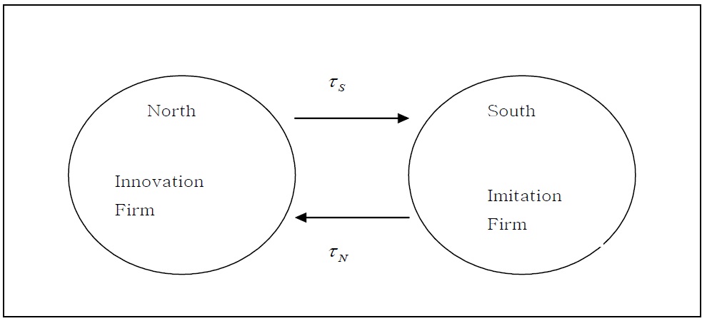
Segerstrom, Anat and Dinopoulos (1990) introduce a North-South trade model to analyze trade policy issues. In their North-South trade model, Northern firms conduct R&D activities to develop higher quality products. These products are initially discovered and produced by firms in the North (developed countries) and are exported to the South (developing countries). Northern firms that innovate receive patent protection for their products and earn monopoly profits until their patents expire. Then production shifts to the South where wages are lower and the products are exported back to the North. They study the steady state equilibrium effects of prohibitive tariffs designed to protect dying industries from competition with Southern firms. These tariffs lead to higher relative wages for Northern workers and a lower rate of innovation in the North. But their model has "scale effects", namely the property that the steady state rate of economic growth is an increasing function of population size. Jones (1995a) criticizes this scale effect property. A variety of endogenous growth models without scale effects have been developed by Jones (1995b), Kortum (1997), Segerstrom (1998), Young (1998) and Howitt (1999).
Sergerstrom and Dinopoulos (2007) adopt an endogenous growth model without scale effects to develop a new North-South trade model. Nevertheless, they left the analysis of tariff imposition in this model as an open question. We extend the North-South trade model developed by Dinopoulos and Segerstrom (2007) by adding tariffs and subsidies and then analyze trade policy using tariffs. We analyze the steady state effects of tariff imposition. Specifically, we study how the tariff imposition and recycling of its tariff revenue (subsidy to domestic firms) of the North (a developed country) or the South (a developing country) affects the innovation rate in the North, imitation rate in the South, wage differential between the two regions, and long-run growth rate of the world economy. Like Dinopoulos and Segerstrom (2007), the innovation only occurs in the North and the South imitates the Northern products. In this paper, Northern firms devote their resources to innovative R&D that enables them to discover higher quality products and Southern firms also devote their resources to imitative R&D that enables them to copy the state-of-the-art quality products. We assume that each government uses its tariff revenue to subsidize domestic R&D. This assumption is based upon the fact that R&D expenditure financed by the government accounts for a substantial percentage in most countries; in particular, 58.6% in Poland, 44.4% in Hungary, and 50.2% in Mexico in 2007 (see Table A1).
We consider the following three cases: first, a tariff imposition only in the South; second, a tariff imposition only in the North; and third, a tariff imposition in both regions. In the first case, we show that a tariff imposition in the South has no effect on the long run growth rate,2 but it leads to a temporary increase in the innovation rate and a permanent increase in the imitation rate. We also show that it reduces wage inequality between the North and the South and leads to higher utility for Southern consumers in the steady state. In the second case, we show that a tariff imposition in the North has no effect on the long-run growth rate, but it causes a temporary increase in the innovation rate and a permanent decrease in the imitation rate. We show that a tariff imposition in the North enlarges wage inequality between the North and the South and leads to higher utility for Northern consumers in the steady state. In the third case, we show that a tariff imposition in both regions temporarily raises the innovation rate, but does not change the long-run rate. The effects on the imitation rate and wage inequality have little effect on the simulation analysis. However, the steady state utility in both regions increased because of quality improvement. The long-run rate of technological change in our model is proportional to the exogenous rate of population growth, and therefore tariffs have no long-run effect, as in other models of economic growth without the scale effect by Jones (1995b) and Kortum (1997).
The rest of the paper is organized as follows. In Section 2, we define our ynamic general equilibrium model of North-South trade with tariffs and subsidies. In Section 3, we identify the steady state conditions for the economy and state the main results. We conclude in Section 4.
1The trade-weighted average tariff for all products of the United States in 2008 was 2%, with 4.1% for agricultural products and 1.9% for non-agricultural products. However, average tariffs vary by industry. In particular, average tariffs were 21.1% for dairy products and 11.4% for clothing. In the case of China, the weighted-average tariff for all products was 4.3%, with tariffs of 10.3% for agricultural products and 4.0% for non agricultural products. Average tariffs were 27.4% for sugars and confectionery and 16.1% for clothing. 2The long-run growth rate or the steady state innovation rate depends only on the population growth rate n and the R&D difficulty parameter λ, as in Segerstrom (1998). The steady state innovation rate is (n/(1-λ)) in this model.
We add tariffs and subsidies to the model of Dinopoulos and Segerstrom (2007). Nevertheless, we will follow the same reasoning as in their paper to derive conditions for steady-state equilibrium.3 There are two regions in the world economy, the North (a developed country) and the South (a developing country). Innovation in the North and imitation in the South take place in the context of trade relations between the two regions. Workers in the North are capable of conducting both innovative and imitative R&D, but workers in the South can only conduct imitative R&D because of the insufficiency of highly trained and specialized labor. In the South, technological progress, or imitation, occurs through the import of product designs and production methods developed in the North.
1. Industry Structure and Quality Improvement
There is a continuum of industries indexed by
In both the North and the South, there is a fixed number of households at each time. Each member of a household lives forever and is endowed with one unit of labor. The size of each household grows exponentially at the fixed rate

population and the South has

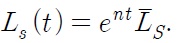
population. The North and the South have the same population growth rate n. Therefore at time t, the supply of labor in the North is
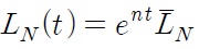
and the supply of labor in the South is

The total supply of labor in the North and the South combined at time
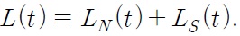
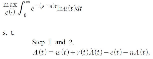
Consumers have identical preferences in the North and the South. Temporal preferences of consumers are given by
where
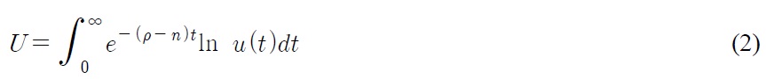
Lifetime utility is given by the discounted sum of the temporal utilities as follows:

where
Each consumer maximizes the lifetime utility by choosing quantities of demand of all types and all qualities. This problem is solved in three steps.
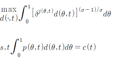
The first step is to solve an industry wide static optimization problem for each industry


where
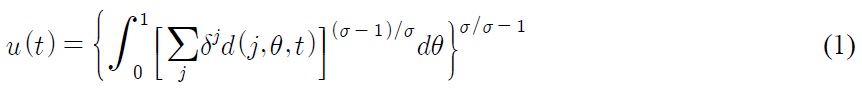
The second step is to solve the cross industry static optimization problem. For each t,

where
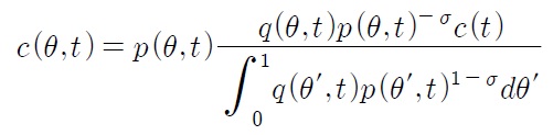
The optimal consumption of
The total spending on

The third step is the inter-temporal expenditure choice problem. Formally:
where

Hence, in a steady state equilibrium, where the expenditure of an individual consumer,
3. Production Technology and Market Structure
Any firm can exit the industry at any time in the North and in the South. Northern firms enter an industry in the North by discovering higher quality products and Southern firms enter by imitating the state-of-the-art products.
There is only one input good, labor, and production technologies of all industries are identical and linear in each region. Northern producers have higher labor productivity than Southern producers. Let
There is an identical production technology across the North and the South, across products, and across quality levels. Goods are produced using one input good, labor, and their production technology exhibits constant returns to scale,
Labor markets are segmented in the North and the South and are perfectly competitive in each region. The wage rate in the North is denoted by
Governments of the North and the South can impose tariffs on imported goods. The tariff rate of the Northern government is denoted by
In any industry, firms (the North or the South) producing different qualities are under the Bertrand price competition. In the case of drastic innovation, the new quality leader immediately charges the unconstrained monopoly price and in the case of non-drastic innovation, the new quality leader charges a limited price initially and immediately reverts to charging the unconstrained monopoly price when he learns that the previous quality leader exited the market. We assume a drastic innovation as in Segerstrom and Dinopoulos (2007).
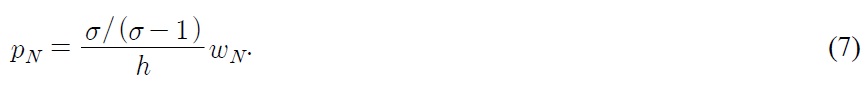
1) Price Determination of Northern Firms
If a Northern firm wins the innovative R&D race, then given the ad-valorem tariff
where
In the Northern market, since the price elasticity of demand for all
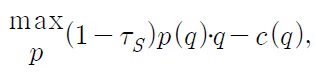
In the Southern market, since Northern firms have to pay a tariff to the foreign (Southern) government when they export the state-of-the-art product to the Southern market, they determine a "pre-tariff" price to maximize the "post-tariff" revenue. Then the Northern firm's profit maximization problem is given as follows: for any

where

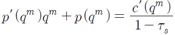
This is the markup condition
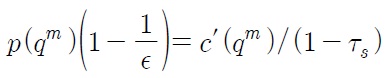
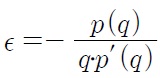
where

is the price elasticity of demand. In this paper, consumers have a constant elasticity of demand

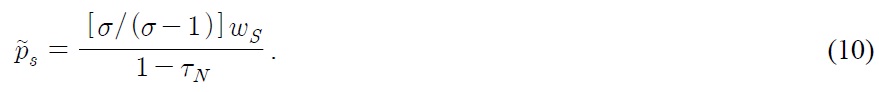
This “pre-tariff” price is the price which the Southern consumer actually confronts. Thus by (7), “post-tariff” price
2) Price Determination of Southern Fir
If a Southern firm wins the imitative R&D race and the North imposes the ad-valorem tariff
where
The Southern firm sets the monopoly price in the Southern market; that is,

And the “pre-tariff” price set by the Southern firm in the Northern market is
Thus by (9), the “post-tariff” price
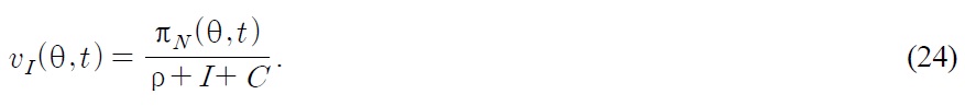
Before deriving an alternative expression for the value of the monopoly profit, we introduce some additional notation. Let

Where
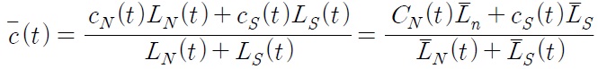
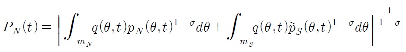
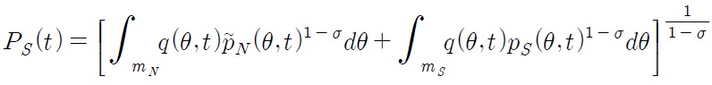
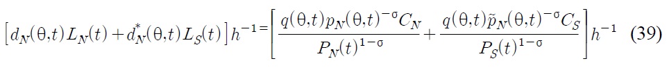
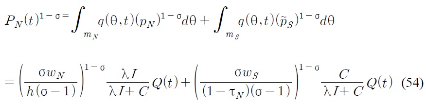
is the global per capita consumption expenditure. In the presence of tariffs, Northern consumers face different prices than Southern consumers and we need to take this into account. Let the Northern quality adjusted price index be defined by

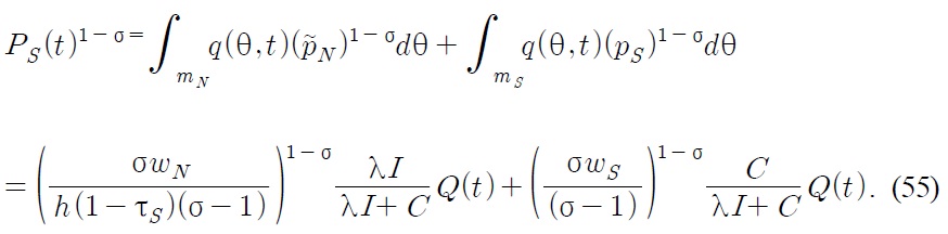
and let the Southern price index be defined by

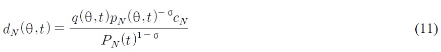
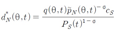
where stars denote exports, subscripts denote production location, is the set of industries with Northern production and is the set of industries with Southern production. Using (3), the Northern consumers demand for a domestically produced good is

The Northern consumer's demand for an imported good (exported by the South) is
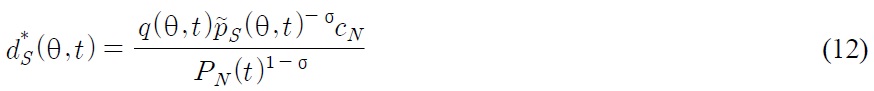
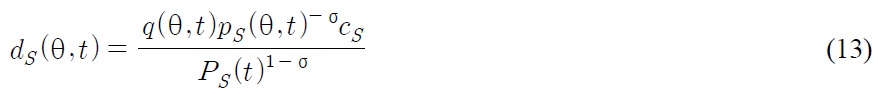
The Southern consumer's demand for a domestically produced good is

And the Southern consumer's demand for an imported good (exported by the North) is
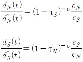
Additionally, we find the following relationship:
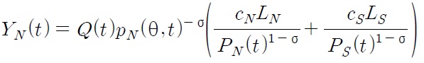
Using the above mentioned notation, a Northern quality leader in industry

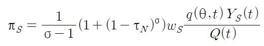
If a Southern quality leader wins imitative R&D, then its profit is given by

4. Innovative R&D and Imitative R&D
Labor is the only factor of production used by firms that engage in either innovative or imitative R&D activities. When Northern firm i hires

where
Southern firms use labor for imitative R&D. When Southern firm

where
The returns to both innovative and imitative R&D's are assumed to be independently distributed across firms, across industries and across time. The probability that some Northern firms innovate in an industry is given by

The probability that some Southern firms imitate in an industry is given by
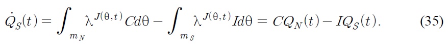
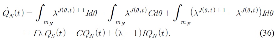
At time t, a measure of

In the steady state, the flow into the industries must be in equal size to the flow out of the industries. If a Southern firm imitates a product of another Southern firm, the profits of both Southern firms become zero because they are involved in the Bertrand price competition. Hence Southern firms imitate the products of Northern firms. If a Southern firm successfully imitates a Northern product, then the production base shifts to the South.7 If a Northern firm successfully innovates a Northern product, this does not cause any shift in the product base. If a Northern firm successfully innovates a Southern product, the production base shifts to the North. Therefore, we obtain the following equation in the steady state.
Using (19), we can derive

All firms maximize expected discounted profits and there is free entry to innovative R&D races in the North. Since all firms have the same innovative R&D technology, a Northern quality leader does not engage in R&D activities. Other firms except the Northern quality leader have incentives to engage themselves in innovative R&D races.
In the steady state, the expected benefit from the innovative R&D is equal to the expected cost. And we assume that the government revenue from the Northern tariff is used to subsidize Northern firms. Let
Firm
Thus, we obtain the following steady state R&D optimization condition:

There is also free entry into all imitative R&D races in the South. In the steady state, the expected benefit from the imitative R&D will be equal to the expected cost. Let
Firm

1) Northern Firms
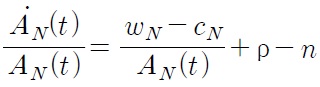
In the stock market, households diversify the risk of holding stocks issued by Northern and Southern firms. Through the no-arbitrage condition, the return from holding the stock of a Northern quality leader must be the same as the return from an equal sized investment in a riskless bond; that is

where
is the dividend rate from the stock of a Northern quality leader,
is the capital gains rate. By the consumer optimization condition, the market interest rate

2) Southern Firms
The stock market value of the Southern quality leader can be similarly derived. The return from holding the stock of a Southern quality leader must be the same as the return from an equal sized investment in a riskless bond. Then, the corresponding no arbitrage condition is
where
is the dividend rate from the stock and

is the capital gains rate. The profits of the Southern quality leader are discounted by the market interest rate. The Southern firm has a possibility to lose its business (i.e. exit the industry) by probability I. The steady state equilibrium reward from imitative R&D is given by

7. Steady State R&D Conditions
1) Northern Firms
Using (21) and (24), we get

Substituting π
The left hand side of (28) is related with the benefit of innovative R&D. The benefit is increasing in
However, the benefit decreases when discount rate ρ, imitation rate of Southern firms
2) Southern Firms
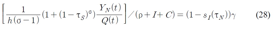
Using (22) and (26), we get

Substituting π
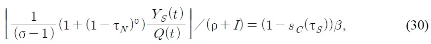
The left hand side of (30) is related with the benefit of imitative R&D. The benefit is increasing in
However, the benefit decreases when the future discount rate ρ or the innovation rate of Northern firms
The average quality of products at time t is given by

where λ = δ(σ–1) > 1. When innovation occurs in industry
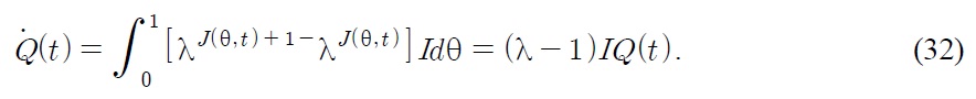
From this equation,
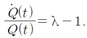
Since the level of relative R&D difficulty

Note that the long-run steady state innovation rate does not depend on the tariff rate, even if the innovation level depends on the tariff rate.
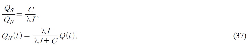
The average quality of all products can be decomposed into the average quality of the Northern leading firms and the average quality of the Southern leading firms as follows:
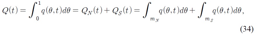
where

The quality of the Northern leading firms improves after successful innovations, but decreases after successful imitations. Then the time derivative of

The growth rates of

1) The Northern Labor Market
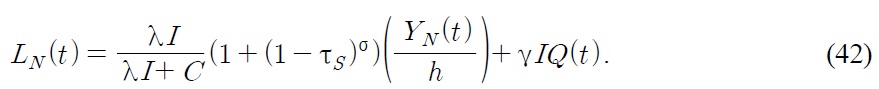
We assume that workers can move freely and instantaneously across firms in the North and the South. In each region, we assume the full employment condition and wage rate is determined by supply and demand in each labor market. The Northern labor demand is composed of two parts, manufacturing employment and R&D employment. Since one unit of product requires one unit of labor, the labor requirement of Northern manufacturing companies equals the world demand for Northern products. Thus the production employment in Northern industry

Since there are leading industries in the North, the total manufacturing labor demand by Northern firms is given by
Northern R&D employment of industry
The labor supply of the North in time

The Northern manufacturing labor demand increases as

(the ratio of Northern products) increases, but decreases as the Southern tariff rate increases. The Northern R&D labor demand is increasing in innovation rare
2) The Southern Labor Market
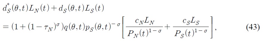
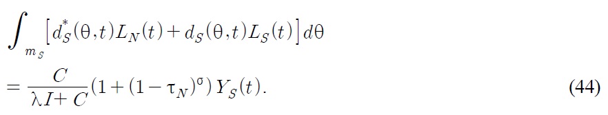
Similarly, manufacturing employment in Southern industry

The total manufacturing employment in the South is given by

Since the Southern R&D employment in industry

And the labor supply of the South at time t is

The Southern manufacturing labor demand increases as
(the ratio of Northern product) increases, but decreases as the Northern tariff increases.
3Specifically, sections 2.1, 2.2, 2.4 follow the same equations as Segerstrom and Dinopoulos (2007). 4. 5. 6This application removes the scale effect of the growth theory criticized by Jones (1995). 7This is called Vernon (1966)’s product cycle model. 8In the steady state condition,
Ⅲ. The Steady State Equilibrium
1. Existence of the Steady State Condition
We determine the Northern steady state condition from the equations (28), (42) and

Similarly, the Southern steady state condition from the equations (30), (46) and

Note that tariff imposition in the South does not affect the Northern steady state condition. It only affects the Southern steady state condition through the subsidy for Southern firms. Also note that tariff imposition in the North does not affect the Southern steady state condition. It only affects the Northern steady state condition through the subsidy for Northern firms.
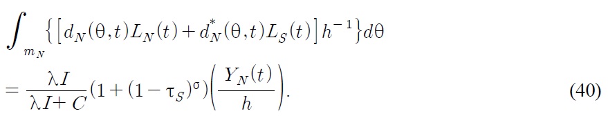
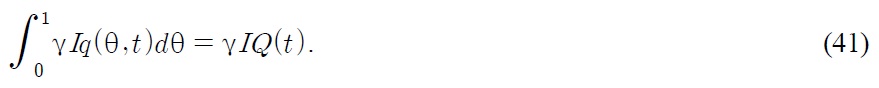
From the two steady state conditions in the two regions, we identify the imitation rate

Thus the quality improves (technology progress) faster as the short-run innovation rate gets higher.
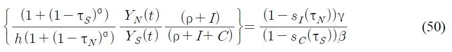
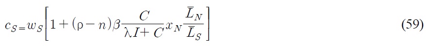
To get the formula for the steady state wage differential

Using (11), (13),

Thus from (50), we can derive the following wage differential equation:
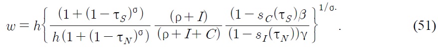
This wage differential equation implies that the North-South wage gap w is indirectly related to the change in tariffs through the change of (ρ +
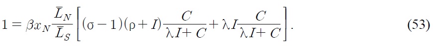
To analyze the effects of a tariff imposition, we compare the equilibrium without a tariff with the equilibrium in the following three cases: first, when only the South imposes a tariff; second, when only the North imposes a tariff; and third, when both regions impose tariffs. From (47) and (48), we obtain the following steady state conditions without a tariff:

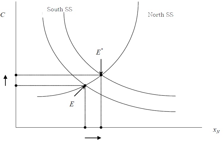
1) Effects of Tariff Imposition in the South
Assume, that there is no tariff in the North and that the South imposes tariff τ
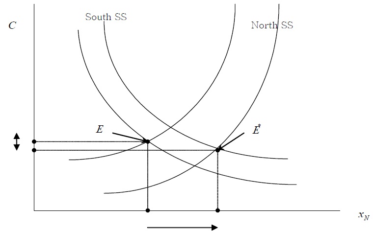
In Figure 2, the steady state equilibrium without a tariff is denoted by
Proposition 1
The steady state of Southern tariff imposition is quite intuitive. The subsidy to the Southern firm from tariff revenue makes imitation R&D more efficient. This leads to more imitation in the South and more industries will move from the North to the South (mN↓, mS↑).
The profit of Northern firm (πN) will decrease caused by the decrease in demand (See 15). The decrease of the profit of Northern firms reduces the R&D benefit of innovation (R&D Reducing Effect) (See 28). On the other hand, the decrease of demand in Northern products leads to a decrease in labor demand in the manufacturing sector in the North (See 39). More Northern workers become available for employment in the Northern R&D sector which makes it more attractive for Northern firms to expand their R&D activities (R&D Enhancing Effect). These two effects offset the Northern steady state equilibrium.
But the industry shift from the North to the South because of the Southern subsidy makes more R&D labor available in the North. Therefore, the short-run innovation rate will jump and technological change will accelerate, but the industry level innovation rate will gradually fall back to the original steady state level
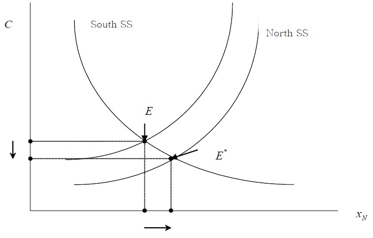
2) Effects of Tariff Imposition in the North
Assume that there is no tariff in the South and that the North imposes tariff τ
After the Northern tariff imposition, the Northern steady state condition curve shifts to the right and the original steady state equilibrium E moves down to a new steady state equilibrium
Proposition 2
The steady state of Northern tariff imposition is also intuitive. The subsidy to the Northern firm from tariff revenue makes innovation R&D more efficient. This leads to more innovation R&D in the North. Therefore, the short-run innovation rate will jump and technological change to accelerate, but the industry level innovation rate will gradually fall back to the original steady state level
The profit of Southern firm π
On the other hand, the more industry shifts from the South to the North, there will be a decrease in labor demand in the manufacturing sector in the South (See 43). More Southern workers become available for employment in the Southern R&D sector. This makes it more attractive for Southern firms to expand their R&D activities (R&D Enhancing Effect). These two effects offset the Southern steady state equilibrium.
3) Effects of Simultaneous Tariff Imposition in the North and in the South
Now assume that both the North and the South impose tariffs on imported goods and subsidize their domestic R&D programs. At that time, both the Northern steady state condition and the Southern steady state condition will change to (47) and (48) (see Figure 4).
In this case, both the Northern steady state curve and the Southern steady state curve shift to the right. The original steady state equilibrium E moves to a new steady state equilibrium
Proposition 3
Let
First, consider how the price indices evolve over time. Using (37), we obtain that
Thus the Northern price index
Thus the Southern price index
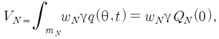
During the lifetime of the firm,

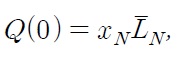
Substituting using (35) and

we determine that the market value of all Northern firms at t=0 is

Using similar notations, the market value of all Southern firms at

Other things being equal, the market value of firms in a region is higher when workers earn higher wages and when innovating is relatively more difficult.
Having determined the market value of the firms, let's solve for consumer expenditures. Let

since the growth rate of

The representative Northern consumer's expenditure is wage income plus interest income on financial assets appropriately adjusted to take into account the splitting of the financial assets that result from population growth. Using (57), the representative Northern consumer's expenditure at the steady state is

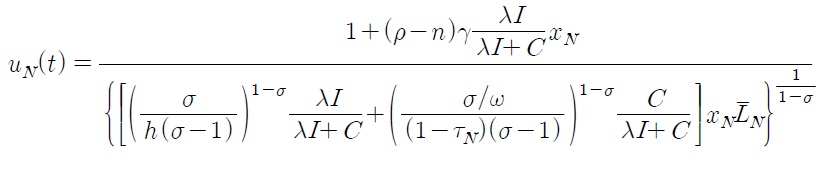
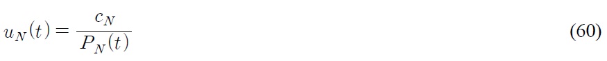
We now turn to the steady state utility paths of representative consumers in the North and South, respectively. For the typical Northern consumer, the utility at time t is

Substituting (11) and (12) yields
From (58) and (54), the steady state utility of the North is

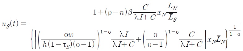
and the corresponding calculations for the Southern consumer yields

From (59) and (55), the steady state utility of the South is

As Dinoupoulos and Segerstrom (2007) identified that, since the old new steady state equilibrium paths involve the same rate of economic growth, we can compare utility levels at time
The results of the simulation analysis should be interpreted as suggestive rather than conclusive, but these results give some implications on the problems which could not be solved analytically. We supposed that the following benchmark parameter values as in Dinopoulos and Segerstrom (2007) were ρ = 0.07,
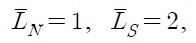
σ = 1.5 and
First, the results confirm proposition 1. According to a tariff imposition in the South,
Second, the results confirm proposition 2. According to a tariff imposition in the North,
Third, the results confirm proposition 3 and show more clearly the undetermined effects. According to a tariff imposition in both regions,
[Table 1] The Result of Computer Simulations
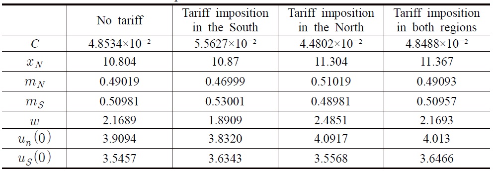
The Result of Computer Simulations
We adopted a dynamic general equilibrium model of North-South trade with scale invariant growth developed by Segerstrom and Dinopoulos (2007) to analyze the steady state effects of tariff imposition. We consider the effects of a tariff starting from a situation of free trade. Assuming that each government uses tariff revenue to subsidize domestic R&D, we showed that tariff imposition in the South leads to more copying of Northern products, faster technological change, lower wage inequality between the North and the South and higher welfare for the Southern consumers. Tariff imposition in the North leads to less copying of Northern products, faster technological change, higher wage inequality between the North and the South and higher welfare for the Northern consumers. Tariff imposition, both in the North and the South, leads to faster technological change and higher welfare in both regions, but has little effect on imitation rate and wage differentials.