There has been some literature that stresses economic policy formation through lobbying and elections. Baron (1994) lets campaign contributions influence the electoral outcome, given the candidates’ platforms. He distinguishes between informed and uninformed voters, assuming that the latter can be influenced by campaign spending. Grossman and Helpman (1996) apply Baron’s model to trade policy formation in which each party is induced to behave as if it were maximizing a weighted sum of the aggregate welfares of informed voters and members of special interests. Bennedsen (2003) extends and simplifies the earlier work by Baron (1994) and Grossman and Helpman (1996). Besley and Coate (2001) study lobbying and elections in a citizen-candidate model. Riezman and Wilson (1997) study the welfare effects of partial restrictions on political competition in a model in which two candidates receive campaigncontributions from import-competing industries in return for tariff protection. Austen-Smith (1987) has an early contribution on the interaction between lobbying and elections. Persson and Tabellini (2000) analyze the provision of public goods using a variant on the model in Bennedsen (2003).

Since most of the papers deal with government spending, the analysis of the equilibrium trade policy through lobbying and elections is rare. Furthermore, this paper is different from the work by Grossman and Helpman (1996), which focuses on the overall effectiveness of campaign contributions when some voters are fully informed and uninfluenced by campaign contributions and other voters are uninformed about economic policy platforms and respond exclusively to campaign contributions. The purpose of this paper is to consider the equilibrium trade policy through lobbying and elections in a small open economy which has a fixed factor of production. Specifically, we consider the economy in which the economic rents exist in the long run because of a fixed factor of production and each interest group has a different share of a specific factor which is used in producing a good. The reason why we assume a fixed factor of production and different share of the factor is the introduction of different economic interests among the interest groups. In fact, the basic model is the simplified version of Grossman and Helpman’s (2005) model, which has three distinct goods and a numeraire good. We build the model of one good because we want to focus on trade policy formation through lobbying and elections. We then examine the equilibrium trade policy in a probabilistic voting model, using Persson and Tabellini’s (2000) approach. We employ the assumption of a small open economy because it is the basis used to analyze equilibrium trade policies and can be easily extended to a large open economy. Also, unlike the previous models by Baron (1994) and Grossman and Helpman (1996), our model assumes that all voters can be influenced by campaign spending.

We have several findings. First, there are no lobbying activities in a probabilistic voting model when both parties announce the same trade policy before elections. Therefore, there is no campaign spending. Second, if all groups are of the same size and organized, or no groups are organized, the equilibrium trade policy is free trade. Third, the different group size and whether or not the group is organized makes the equilibrium trade policy different from free trade when the number of swing voters is the same in each group.

The organization of the paper is as follows. In the next section, we develop the model and set up a small open economy which has a fixed factor of production. We then introduce the indirect utility of an individual in the economy. In section Ⅲ, we derive the preferred policy of an individual in the economy and formulate the utilitarian benchmark to compare it with the equilibrium trade policy in the probabilistic voting model with lobbying in the following section. In section Ⅳ, we introduce the probabilistic voting model with lobbying, derive the equilibrium trade policy in that model and then compare it with the utilitarian benchmark. Section Ⅴ offers our conclusions.

Consider a small open economy populated by a large number of citizens, where the size of the population is n. These individuals consume a good and are of different types indexed by i. The good is manufactured from an industry-specific factor with constant returns to scale. The specific input is available in an inelastic supply. We let ∏(p) represent the aggregate rent accruing to the specific factor used in producing the good.1 Then the slope of this function gives the industry supply curve

where p is the domestic price of the good.2 The domestic price p of the good is the sum of the given international price p^* and the specific import tariff or import subsidy τ.3

To make the arguments more clear, we adopt linear forms for the supply and demand functions. The supply function is given by

where x^* is the quantity of the good produced at the free-trade price and γ is the non-negative parameter.4 It reflects the fact that the domestic quantity of the good produced when the domestic price is equal to the international price is the same as the quantity of the good produced at the free-trade price. Furthermore, the higher the import tariff, the greater the domestic quantity of the good produced and vice versa. The demand function is given by

where d^* is the quantity of the good consumed at the free-trade price and β is the non-negative parameter.5 It also reflects the fact that the domestic quantity of the good consumed when the domestic price is equal to the international price is the same as the quantity of the good consumed at the free-trade price. Furthermore, the higher the import tariff, the smaller the domestic quantity of the good consumed and vice versa.

Let individual i own a different fraction of the specific factor denoted by αⁱ. We also assume that everyone has the same demand function. Then, it implies that his indirect utility is given by

where Iⁱ is individual i’s income of rents and transfers, CS(p) is total consumer surplus from consumption of the good, and m( p) = d(p) - x(p) is the quantity imported.6 Note that -CS’(p) = d(p) is the demand for the good. We assume that αⁱ is distributed in the population according to a cumulative distribution function F(ㆍ). The expected value of αⁱ is denoted by

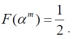
Finally, the median value of αⁱ , denoted by α^m , is implicitly defined by

1Varian (2003) describes economic rent as those payments to a factor of production that are in excess of the minimum payment necessary to have that factor supplied. One of the examples he suggests is oil. The reason why oil sells for more than its cost of production and firms don’t enter this industry is the limited supply. Since only a certain amount of oil is available, there are a fixed number of firms in the market though they try to enter.  2The number of firms in the industry is fixed because there is a factor of production that is available in fixed supply. In this case, the equilibrium rent in competitive market will be whatever it takes to drive profits to zero; pe xe - z (xe) -∏ = 0 or ∏(pe ) = peㆍ x (pe) - z (x ( pe )) , where z is the variable cost of producing the good and the e superscript represents the equilibrium levels. Furthermore, ∏’( pe ) = x ( pe ) + peㆍ x’( pe ) - z’(x ( pe ))ㆍ x’( pe ) = x (pe) + ( pe - z’(x ( pe )))ㆍ x’( pe ) = x ( pe ) , since pe = z’(x ( pe )) in competitive market. Grossman and Helpman (2005) use this kind of setup with four goods, a numeraire good and three distinct goods.  3If τ > 0 , we call it an import tariff; if τ < 0 , we call it an import subsidy.  4Since rises as γ increases in both cases of p - p* > 0 and p - p* < 0 .  5Since rises as β increases in the case of p - p* > 0 and rises as β increases in the case of p - p* < 0 .  6policymaker sets τ , taking into account the market-determined value of p and some further constraints, such as a balanced government budget constraint or a resource constraint. Typically, the constraints will be binding; that is, the market outcomes depend on policy variables and parameters.

In this section, we compute individual i ’s preferred policy and provide the utilitarian benchmark. This will be useful in the next section in which we compute the policy level in the voting equilibrium and compare it with the utilitarian benchmark.

Individual i maximizes his indirect utility;

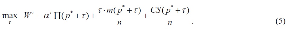
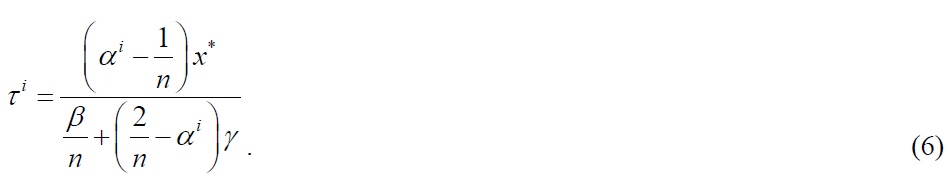
Using expression (5), it is straightforward to obtain the first-order condition, which becomes his preferred policy or his bliss point by Assumption 1 below (see Appendix A);

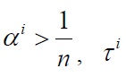
Assumption 1 β > 2(αⁱ n -1)γ, ∀αⁱ.

This implies that everyone’s demand responds to the change in τ sufficiently large enough that β > 2(αⁱ n -1)γ. Since W(τ ;αⁱ ) has a quadratic form, this assumption is needed to make sure that individual i has the maximum at his bliss point. We also need this assumption to show that the median-voter theorem holds. With this assumption, there are two interesting properties derived from the bliss point of individual i First, individual i, who has the bigger share of the specific factor, prefers higher protection because τ(αⁱ) is increasing in αⁱ.7 Second, the sign of τⁱ depends on the size of αⁱ. On the one hand, if

is positive. It means that in dividual i, who has the share of the specific factor greater than

likes an import tariff. On the other hand, if

is negative. It means that individual i, who has the share of the specific factor less than

likes an import subsidy. If, of course, individual i, who has the share of the specific factor equal t

prefers free trade.

Next, let us formulate a normative benchmark to compare it to the trade policy level in the voting equilibrium. Consider a utilitarian social welfare function that simply integrates over the welfare of all individual citizens:

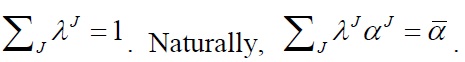
where the last term is the utility of the individual with the average share of the specific factor. This equality follows from the definition of Wⁱ (ㆍ) and the fact that

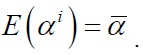
Namely,

The first order condition is

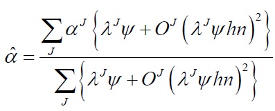
which gives

where the so superscript stands for the socially optimal level. According to the utilitarian objective, the socially optimal policy coincides with the policy desired by the citizen who has the average share of the specific factor. Furthermore, this trade policy is free trade because

7

In this section, we introduce the probabilistic voting model encompassing campaign contributions by interest groups, adapting a formulation suggested by Baron (1994).8 We postulate two candidates or parties indexed by P = A, B. Each of these maximizes the expected value of some exogenous rents, R. Candidate P sets his policy so as to maximize P_q ㆍ R, where P_q is the probability of winning the election, given the other candidate’s policy. If we use π_p to denote the vote share of candidate P, we can write

We assume that the population consists of three distinct groups, J = H,M, L, representing the high, the middle, and the low share of the specific factor, respectively. Each group’s share of the specific factor has the obvious ranking:

and everyone in group J has the same share of the specific factor. The population share of group J is λ^J, with

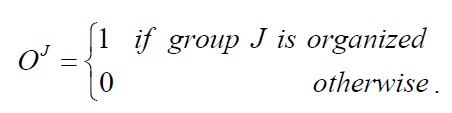
We assume that groups may or may not be organized in a lobby; the indicator variable O^J takes a value of one if group J is indeed organized, zero otherwise;

Organized groups have the capacity to contribute to the campaign of either of the two candidates: let C^J_P denote the contribution per member of group J to candidate P, constrained to be nonnegative. These contributions can be interpreted as both in cash and in kind. The total contributions collected by candidate P can thus be expressed as

At the time of elections, voters base their voting decisions both on eco-nomic policy announcements and on the two candidates’ ideologies. Specifically, voter i in group J prefers candidate A if

where σ^iJ is an individual-specific parameter that can take on negative as well as positive values. We assume that this parameter has group-specific uniform distributions on

We also assume that candidates exploit the contributions in their campaign and that campaign spending affects their popularity. Specifically, the average relative popularity of party B, δ, has two components:

where

is distributed uniformly on

According to the second term, a candidate who outspends the other becomes more popular, where the parameter h measures the effectiveness of campaign spending. C_B might measure advertising expenditures or media exposure of party B’s leaders, but it might also refer to support actions in favor of party B’s candidate or against her electoral opponent.

The timing of events is as follows. At stage one, the two candidates, simultaneously and noncooperatively, announce their electoral platforms: τ_A τ_B. At this stage, they know the voters’ policy preferences and the distributions for σ^iJ and δ. At stage two, the contributions are given simultaneously by all lobbies, and then the actual value of δ is realized and all uncertainty is resolved. At stage three, elections are held. Finally, the elected candidate implements his announced policy platform.

To formally study the candidates’ decisions at stage two, let us identify the swing voter in group J, a voter whose ideological bias, given the candidates’ platforms, makes him indifferent between the two parties:

All voters i in group J with σ^iJ≤ σ^J prefer party A. Hence, given our distributional assumptions, candidate A’s actual vote share is

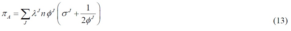
Specifically, candidate A’s probability of winning, given (12), becomes

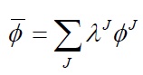
where

is the average density across groups (see Appendix B).

Assumption 2 ϕ^J = ϕ for all J.

This implies that all groups have the same density, ϕ, making the members of each group, in their capacity as voters, equally attractive for office-seeking politicians. Then (14) becomes

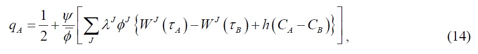
where

is the utilitarian social welfare function (see Appendix B). The last term reflects how campaign spending has an influence on the expected vote share.

Consider how lobbies choose their campaign contributions at stage two. If organized, group J chooses contributions with the objective of maximizing the expected utility its members derive from the election, minus the cost of contributions:

The first two terms in the expression are the expected utility group J ’s members derive from the election. The negative third term can be interpreted in two ways. If transfers are made in cash, this could reflect the increasing marginal costs of enticing potential contributors with different willingness to give, which makes the costs convex. If transfers are made in kind, such as work in the campaign, the convexity may represent the increasing disutility of effort.

Maximization of (16) with respect to C^J_A and C^J_B, subject to (15), yields group J’s optimal contributions:

Thus each group contributes only to the candidate whose platform gives the group the highest utility, and does not campaign at all if the two parties announce the same platforms.

We now return to the candidates and their optimal platform choice at stage one. When making this choice, the candidates anticipate that organized groups will make contributions according to (17) and (18). But the symmetry of (17) and (18) preserves the symmetry of the two candidates’ problems. Thus, they converge on the same equilibrium policy. To characterize this policy, we substitute (17) and (18) into (15) and simplify. Candidate A , taking τ_B as a given, maximizes

By the same logic, party B solves an identical problem. Hence, both parties announce the same policies, τ_A = τ_B, which then implies that equilibrium campaign spending is zero.

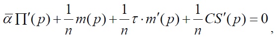
However, out of equilibrium, they do spend on the party that pleases them most, and this induces both parties to tilt trade policy in their favor. To see when only a subset of the groups is organized, we take the first-order condition of (19) with respect to τ_A. After some arrangements we get:

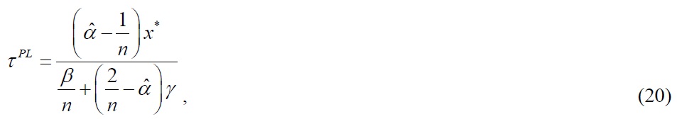
where

and the PL superscript stands for the equilibrium in a probabilistic voting model with lobbying (see Appendix C). The equilibrium trade policy has weights reflecting group size and whether or not the group is organized. With this equilibrium trade policy, we have the following proposition.

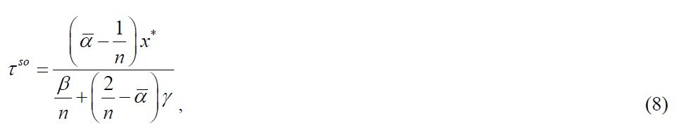
Proposition 1 can be explained as follows. The intuition that the equilibrium is socially optimal when all groups are organized is that the groups are all prepared to contribute in proportion to the marginal benefits and costs of τ for their members. As a result, the candidates internalize all groups with the appropriate social weight.10 In case of no organized groups, we also get the social optimum since there are no social wastes.

Except in the conditions specified in Proposition 1, the organized groups receive greater weights and the equilibrium is tilted in their favor. Furthermore, even though the number of swing voters is the same in each group, the group size (λ^J ) and whether or not the group is organized (O^J) make the equilibrium trade policy different from free trade. Now we consider several possible cases. First, we assume λ^H > λ^M > λ^L , so that the group with the low share of the specific factor has the smallest size. In this case, even though all groups are organized,

implying an import tariff that is in the equilibrium. For the given α , the bias is larger when the group with the high share of the specific factor is larger – as more campaign spending can be possible - and the higher it is relative to the group with the middle share of the specific factor (α^H -α^M larger) – as the group with the high share of the specific factor then has a higher stake in the policy. Second, we assume λ^H > λ^M > λ^L, so that the group with the low share of the specific factor has the largest size. In this case, even though all groups are organized,

implying an import subsidy that is in the equilibrium.

Proposition 2 can be explained as follows. If the group with the high share of the specific factor has the largest size and is organized, it has the highest stake in the policy. Thus, both candidates announce a platform with a trade policy which is favorable to them.

8Yang (2008) examines the voting and elections without lobbying.  9The first-order condition of the lobby J with respect to CJA is The first-order condition of the lobby J with respect to CJB is   10Note that big groups are favored if they are organized. The reason is that the marginal cost of lobbying is increasing, and lobbying is a public good for the group. Big groups can spread the same amount of contributions over more members, who thus face a smaller marginal cost and are willing to lobby more.

We have considered the equilibrium trade policy through lobbying and elections in a small open economy which has a fixed factor of production. Rents exist in this economy because the factor of production has a fixed supply even in the long run. Individuals have different endowments of the factor of production and rents from each individual’s share of the factor are a part of his income.

We have shown that there are no lobbying activities in the probabilistic voting model when both parties announce the same trade policy before elections. In the game specified in the model, neither group has an incentive to lobby the candidates when they announce the same trade policy before elections. We have also found that if all groups are of the same size and are organized, or no groups are organized, the equilibrium trade policy is free trade. Since the groups contribute in proportion to the marginal benefits and costs of trade policy for their members, the candidates internalize all groups with the appropriate social weight. Finally, we have found that even though the number of swing voters is the same in each group, the different group sizes and whether or not the group is organized can make the equilibrium trade policy an import tariff or an import subsidy.

A further extension of this paper is a model that considers different inter actions between two different types of political activities, such as elections and legislative bargaining, lobbying and legislative bargaining.11 It will be interesting to see how the equilibrium trade policy changes as we introduce different interactions in political activity. By introducing those, we can gain a better understanding of how the policy is formed in different economic circumstances.

11Yang (2010) analyzes the legislative bargaining over trade policy without lobbying after elections.