The Earth is surrounded by two well-known radiation belts, the inner and outer belts, both containing high energy charged particles. The two belts are separated by the slot region. The inner belt is relatively stable, and the outer belt suffers from substantial changes due to various reasons (e.g., Kim et al. 2011, Lee et al. 2013). The outer belt variations include the long-term solar cycle-dependent variation (Li et al. 2011, Lee et al. 2013), an immediate response on a minute time scale when the magnetosphere is directly hit by solar wind shock (Li et al. 1993), and the more usual variations on an intermediate time scale, typically hours to days. The currently prevailing view for the physical reason responsible for such variations is largely, though not necessarily exclusively, based on the global transport and the more local wave-particle interaction. The observed flux at a given time and location by a satellite is a net result of delicate balance between the acceleration (source) and loss effects (Reeves et al. 2003).
The plasma sheet supplies the seed electrons and ions particularly under the enhanced convection, substom and storm times. The transported electrons themselves become the radiation belt components after acceleration by plasma waves as well as by radial diffusion process. The most responsible plasma wave for acceleration is believed to be whistler chorus usually identified outside the plasmasphere (Horne & Thorne 2003). The chorus waves can also act to scatter electrons to precipitate into the upper atmosphere (Horne & Thorne 2003, Lam et al. 2010). Other waves such as electromagnetic ion cyclotron waves and plasmaspheric hiss waves can also contribute to atmospheric loss (Summers & Meredithet al. 2007 Kim et al. 2011). The electrons can also be lost into the solar wind through magnetopause crossing under stressed condition by solar wind (Kim et al. 2008, 2010, Turner et al. 2012, Hwang et al. 2013). The electron flux dropout has also been attributed to magnetic field line stretching (Onsager et al. 2002, Lee et al. 2006).
Quantitative specification of all these effects is the main trend of the present day research in this field. On one side, observations by satellites such as CRRES (e.g., Meredith et al. 2000) and more recent Van Allen Probes (e.g., Baker et al. 2013) have improved our understanding of the outer radiation belt dynamics in terms of acceleration and loss effects. On the other side, the radiation belt researchers have long been trying to model the outer belt variations (See a review by Shprits et al. 2008). A simple model is based on the radial diffusion of electrons across drift shells over time scales of hours-to-days after being transported from the plasma sheet. However, a comparison with observations indicated that the radial diffusion alone cannot fully explain the observed flux distribution in the outer belt (Miyoshi et al. 2003). It became soon evident that local acceleration effect needs to be taken into account. Presently existing physical models of the radiation belts solve a fully three dimensional, even four dimensional equation of diffusion and transport (e.g., Fok et al. 2008, Shprits et al. 2009). These models include the local diffusion in energy (or momentum) and pitch angle, radial diffusion across drift shells, and the transport from the plasma sheet. Determination of the diffusion coefficients and transport effect for each responsible process is critical and remains a major research topic.
In the present paper, we adopt a strategy to model the outer belt electron distribution based on the radial diffusion equation with observationally determined specifications of a few critical factors. We use observationally determined functional forms for the outer edge boundary conditions and plasmapause locations. Most importantly, we modify the radial diffusion equation by incorporating chorus effect as a source term in an empirical way. We present a comparison between the results with and without the chorus effect and demonstrate the effectiveness of our simple model. The main purpose of this paper is to give a description of the essence of this new model.
2. PHYSICAL STRUCTURE OF THE MODEL
Our model is based on the one-dimensional radial diffusion equation that is modified by inclusion of a term representing the chorus effect,
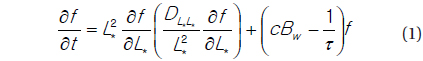
where
First, for the diffusion coefficient

This reflects a temporal dependence in an implicit way via time-varying
Second, formally Equation (1) is an initial value and boundary condition problem. In particular, the radiation belt electron fluxes are strongly affected by the energy spectrum of the electron flux at the outer boundary. If local acceleration and loss effects are ignored, the radiation belt structure is determined entirely by radial diffusion process which is subject to the boundary condition. Thus specifying the outer boundary condition in a precise way is critical. To set the energy spectrum of the electron flux at the outer boundary of the belt, we use the functional forms that we have recently determined using the observations of energetic electrons by solid state telescope on THEMIS (Shin & Lee 2013). In these functions, the boundary fluxes of electrons at various energies (from 30 keV up to 719 keV) at r = 7-8 RE on the nightside are expressed in terms of past solar wind speed and density. The details of the results are reported in Shin & Lee (2013) – See Table 2 and Fig. 8 in Shin & Lee (2013). An alternative option that we can choose for description of the boundary conditions is to use the energetic electron fluxes measured by GOES 13 or 15 satellites on geosynchronous orbit. We have recently developed a separate neural network-based scheme to predict electron fluxes at geosynchronous orbit by up to 24 hours -- See Ling et al. (2010) for an example of an application of the neural network technique to geosynchronous electron flux data. This can be used to set the outer boundary conditions as well, but a drawback is that the differential fluxes of electrons are obtained only for 40 keV to 475 keV and one needs an extrapolation to higher energy. Our empirical specification of the outer boundary condition implicitly takes into account the effects due to the drift loss and transport from the plasma sheet.

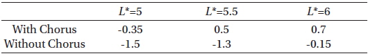
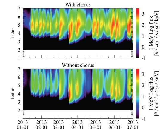
Comparison of prediction efficiency between the diffusion results with and without chorus.
Third, it is well known that the atmospheric loss time scale τ differs between the regions inside and outside the plasmasphere due to different scattering mechanisms. Therefore, for example, Shprits et al. (2005) set it to be 10 days inside the plasmasphere and scaled it by 3/
Fourth, to specify the chorus term which is the most important part in the equation, we first determine the global distribution of chorus wave intensity. We use the THEMIS satellite observations for the interval of about 4 year period from July 2007 through July 2012 excluding the year 2009 when the solar wind conditions and the magnetospheric activities were unusually weak (Lee et al. 2013). Specifically we use the filter bank data of Search Coil Magnetometer (SCM) onboard the THEMIS satellites (Roux et al. 2008). Our method to identify chorus is basically the same as in the previous work by Li et al. (2010). Specifically, we use the data at top three frequency ranges (1390-4000 Hz, 320-904 Hz, 80-227 Hz) out of the six bands of the filter bank data (Cully et al. 2008). Events with the known noise level of 4 pT or less are excluded. We assume that
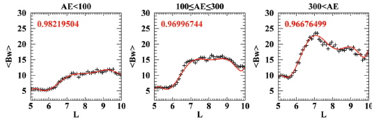
Li et al. (2010) report the global distribution of the chorus amplitude for a similar data set, and we obtain similar results (see Fig. 2 in this paper). Thus we do not repeat to present this in this paper. The main advance in our work is that we have developed a prediction model for a global distribution of chorus intensity. Our chorus model is capable of predicting the chorus intensity by 30 minutes using the z-component of the interplanetary magnetic field and the geomagnetic index AE. The prediction can even be made separately for the near equator region (|magnetic latitude| ≤ 10°) and for the region away from the equator (10° < |magnetic latitude| ≤ 25°). The details of this chorus prediction model will be reported elsewhere (Kim JH et al., A prediction model for the global distribution of whistler chorus waves including latitudinal dependence, Manuscript submitted to JGR 2014). The present version of our radiation belt model does not fully make use of this sophisticated function of the chorus prediction model. Rather our strategy for the present radiation belt model is to employ a simplified version of the chorus model that can be easily incorporated into the diffusion Equation (1).
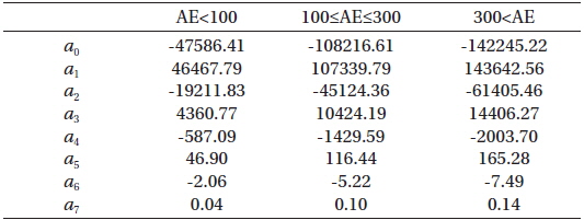
Specifically, we first obtain the magnetic local time (MLT)–averaged, but
[Table 1.] Coefficients of fit functions for chorus intensity.

Coefficients of fit functions for chorus intensity.
where
Last, we determine the calibration factor
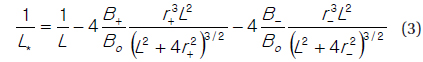
Fig. 2a shows the observationally identified plasmapause locations

where
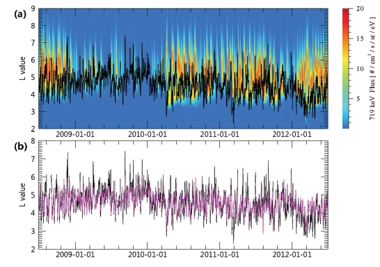
In Fig. 3 we present the results of application of (1) to a new interval. The panels (a) and (b) in Fig. 3 show the predicted fluxes of 1 MeV electrons with and without the chorus term, respectively. The difference between the two simulation results in Fig. 3 is clear enough to identify that the flux enhancement at the central region of the outer belt is more pronounced when the chorus effect is included. Elsewhere the chorus effect appears to make no significant difference. Also there is no major difference in the inner boundary position of the outer belt between the two simulations. We estimate the prediction efficiency of each model result with the observations made by the Van Allen Probes. Table 2 shows the results for selected
In this paper, we described the physical formalism of the outer radiation belt model that we have recently developed at Chungbuk National University. The model is based on the simple, mathematically one-dimensional, but physically higher dimensional, equation of diffusion. We have determined three main factors observationally that affect the solution of the diffusion equation. They are the boundary condition at the outer edge of the outer belt, the plasmapause location, and the chorus acceleration effect. The developed model captures the flux enhancement at the central region of the outer radiation belt to some reasonable degree. While, for a more rigorous treatment of diffusion physics, one has to rely on a more “expensive” three dimensional diffusion equation (e.g., Shprits et al. 2009), our simplified model is more suitable for space weather forecast purpose. Improvement of the effects included here and further addition of other effects will further enhance the accuracy of the model.
We plan to improve our model in the following aspects. First, we will develop a better scheme for the