The surface of the Moon is covered with millions of impact craters due to the fact that there is no atmosphere on the Moon to protect it from collisions by asteroids, comets, or meteorites. These celestial objects hit the Moon at a wide range of speeds, about 8 to 20 km/s. Also, there is no erosion phenomena and little geologic activity to wear away these craters, so they remain unchanged until another new impact changes it. These facts and others led the celestial dynamists and geophysicists, over the years, to conclude that the Moon's gravity is stronger in some regions than others, creating a lumpy gravitational field. In particular, impact basins exhibit unexpectedly strong gravitational pull. Scientists have suspected that the explanation has to do with an excess distribution of mass below the lunar surface, and have dubbed these regions mass concentrations, or “mascons”. These collisions send material flying out, creating a dense band of debris around the crater’s perimeter. The impacts send a shockwave through the Moon’s interior, reverberating within the crust and producing a counter wave that draws dense material from the lunar mantle toward the surface, creating a dense centers within the craters. See the URL, http://newsoffice.mit.edu/2013/an-answer-to-why-lunar-gravity-is-so-uneven-0530 and for more details see Melosh, et al. (2013).
The physical exploration of the Moon began when Luna 2, a space probe launched by the Soviet Union, made an impact on the surface of the Moon on September 14, 1959. In 1969, NASA's Project Apollo first successfully landed humans on the Moon. They landed scientific instruments on the Moon and returned lunar samples to the Earth. In 1966, Luna 9 became the first spacecraft to achieve a controlled soft landing, and Luna 10 became the first mission to enter orbit.
Between 1968 and 1972, manned missions to the Moon were conducted by the United States as part of the Apollo program. Apollo 8 was the first manned mission to enter orbit in December 1968, and was followed by Apollo 10 in May 1969. Six missions landed men on the Moon, beginning with Apollo 11 in July 1969.
Also in last decade, on September 14, 2007 Japan launched an artificial satellite around the Moon. China also launched a lunar satellite on October 24, 2007. Both countries have participated in many missions to the Moon in this decade. Also, India launched a lunar orbiter (Chandrayaan 1) on October 22, 2008, for two-year mission aimed to map the Moon, Carvalho et al. (2010). This competition motivate the researchers from all countries to focus on the orbits of lunar orbiters.
The motion of an artificial satellite around the Moon is quite different from the one around the Earth on several aspects. The most important difference is that the Moon is a slowly rotating body. Secondly the Moon's atmosphere has nearly negligible effect on the motion of the Moon's satellite in contrast to that of the Earth. It is also well known that, the lunar gravity field is far from being central, nor does it exhibit any strong symmetry of revolution; the order of magnitude for the Earth spherical harmonics can be found in Kaula (1966), see e.g. Konopliv et al. (2001) for a recent model in spherical harmonics, and for the Moon, Bills & Ferrari (1980).
The Moon is much less flattened than the Earth, which makes the C22, the first sectorial harmonic coefficients, come closer to J2, the first zonal harmonic coefficients; so this needs to be considered. Moreover, the effect of the Earth on the lunar satellite is much larger than the effect of the Moon on a terrestrial satellite; so the former effect is combined into the effects of the shape of the lunar gravity field.
In this paper, we will focus on the combined effect of the lunar perturbing terms factored by J2=-202×10-6, C22=22.26×10⁻⁶ and/or C31=28.43×10⁻⁶; the first tesseral harmonic coefficients, on the critical inclination of a lunar artificial satellite.
The value of inclination that enforces the rate of argument of periapsis change of an orbit under the effect of considered perturbations to be equal zero is called critical inclination IC. This phenomenon of the critical inclination in the Earth artificial satellite theory has been known since 1950’s. In-depth overview and an extensive list of related papers can be found in Coffey et al.(1986, 1994). The first order secular perturbations in the argument of pericentre vanishes at the critical inclination, but when the second order approximation is used the phenomenon clearly becomes a resonance problem.
In the Earth artificial satellite theory, the critical inclination under J2- perturbation is well known to be 63.43° for direct orbits or 116.47° for the retrograde orbits. Due to the importance of IC applications in the Earth’s satellite orbits; Molniya orbit type as a communication satellite at Earth's high latitude is aimed, it attracted many research attentions, and here are more works relevant but not limited.
Delhaise & Morbidelli (1993) investigated the luni-solar effects on a geosynchronous satellite in near the critical inclination. Yi & Choi (1993) studied the characteristics and perturbation effects on the artificial satellite orbit with critical inclination. Abd El-Salam & Ahmed (2005a,b) discussed Post-Newtonian (PN) effects on the critical inclination angle in the Earth artificial satellite theory including the zonal harmonics up to J4 and the PN contributions up to order J2/c2; c is the velocity of light. Breiter & Elipe (2006) reformulated IC in traditional Earth's artificial satellite theory to have an arbitrary satellite's mass and the tilted rotation momentum vector with respect to planet symmetry axis.
On the other hand, the dynamics of lunar orbiters is quite different from that of an artificial Earth satellite in which the Moon is less flattened than the Earth, that cause C22/J2 is only 0.1; where C22, the first sectorial harmonics coefficient. Thus researchers introduced different studies to calculate the effects of such a difference on IC of the Moon orbiters; for example, De Saedeleer & Henrard (2006) found that the IC is strongly affected by the C22 coefficient and by the value of the longitude of the ascending node, Ω. De Saedeleer (2006) investigated an analytical theory of a lunar artificial satellite with third body perturbations(Tzirti et al. 2009) declared that the inclination does not remain constant but in long periodic oscillations taking in consideration the effect of J2 and C22 harmonics(Carvalho et al. 2009) studied second order critical inclination and presented a new formula to compute inclinations for Sun-synchronous orbits under the effect of J2 and C22 harmonics(Carvalho et al. 2010) studied the effect of non-uniform mass distribution of the Moon in addition to effect of Earth as a third-body on the lunar orbiter(Liu et al. 2011) studied Venus's IC and they found in general the IC may have multiple solutions(Carvalho et al. 2010) presented an analytical theory with simulations to study motion of lunar low-altitude spacecraft. Also many studies were made for lunar frozen orbits (Elipe & Lara 2003, Folta & Quinn 2006, Park & Junkins 1995) to make the orbiter pass by a given latitude with the same altitude by keeping the argument of the periapsis and the eccentricity of the orbit constant. Rahoma et al. (2014) calculated the effects of PN corrections in addition to C22 for an Earth-like planet supposing all considered perturbations of the same order of magnitude.
The flatness of the Moon is less than the Earth which makes the C22 coefficient closer to the J2 and the next important one to be considered is C31, which is the core of this study.
In this study, the effect of C31 on IC is computed in Hamiltonian framework considering C31, C22, and J2 of the same order of magnitude; that is of order 𝒪(1). In addition, numerical simulations are introduced. The Moon's flatness has C22/J2 only 0.1 and C31/J2≅0.14, so the most important harmonic to be considered other than J2 and C22 should be C31. It is also observed that . In order to calculate the families of critical inclinations, the short period terms are eliminated using Delaunay canonical variables after the Hamiltonian of the problem is constructed,.
Our results can be applied to a special type of orbit, a Sun-synchronous orbit for Moon’s artificial satellites. The Sun-synchronous orbit is a particular case of an almost polar orbit. The satellite travels from the North Pole to the South Pole and vice versa, but its orbital plane is always fixed for an observer that is posted in the Sun. Thus the satellite always passes approximately on the same point of the surface of the Moon every day in the same hour. In such a way the satellite can transmit all the data collected for a lunar fixed antenna, during its orbits. An analysis of Sun synchronous orbits considering the non-uniform distribution of mass of the Moon is done for the longitude of the ascending node with an approach based on Park & Junkins (1995).
To achieve our goal, this paper is organized as follows. In Section 2, the potential of the Moon is presented and the Hamiltonian of the system is constructed using Delaunay canonical variables. In Section 3 and Section 4, we eliminated the short periodic terms from the Hamiltonian and we obtained the new families of critical inclinations using a single-average procedure. In Section 5 and Section 6, we gave numerical simulations and discussions on the results. Finally, in Section 7 a conclusion is presented to draw attention about the importance of C31 effect on the value of critical inclination for the bodies that have uneven mass distribution like the Moon.
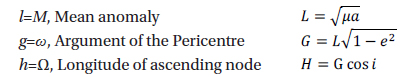
In the main problem, the following approximations are made by Giacaglia et al. (1970): i) the Moon's orbit around the Earth lies on the lunar equatorial plane; ii) the orbit of the Moon around the Earth is circular; iii) the longitude of lunar longest meridian λ22 is equal to the longitude of the Earth λ⊕. The classical Keplerian orbital elements are used to define the orbit of a lunar orbiter; i.e. semi-major axis a, eccentricity e, inclination i, argument of the periapsis ω, longitude of the ascending node Ω, and the true anomaly f. Also n and are the mean motion and the radius vector of an orbiter from the center of the Moon.
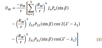
Using the lunar equatorial plane as the fundamental plane, then lunar disturbing potential per unit mass can be written as (d’Avanzo et al. 1997, Radwan 2002)
where μM is the lunar gravitational constant, RM is the equatorial radius of the Moon, Pn, Pnm are the Legendre polynomials, the angle β is the latitude of an orbiter with respect to the equator of the Moon, the angle λ is the longitude measured from the direction of the longest axis of the Moon, the angle λ' is its longitude reckoned from any fixed direction. (r,λ,β) is the lunar centric coordinates of the orbiter , and λ2 is the longitude of the Moon’s longest meridian reckoned from the same fixed direction, and clearly λ2 depends explicitly on the time through the relation λ2=λ2 (0)+υMt where υM is the spin speed of the Moon about its axis.
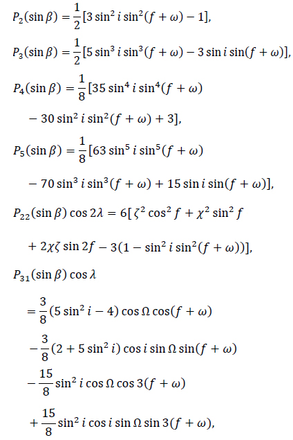
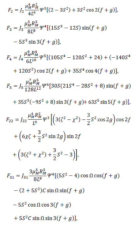
The leading harmonics of lunar potential are almost of the same order, this complicates the choice of the harmonics at which the potential may be truncated and makes the choice somewhat arbitrary. In terms of the orbital elements the Legendre terms will now be (El-saftawy, 1991)
where
ζ = cos ω cos Ω – cos i sin ω sin Ω,
Χ = -sin ω cos Ω – cos i cos ω sin Ω
The Hamiltonian F depends explicity on the time through its explicit appearance in λ2. Suppose λ2=λ⊕; where, λ⊕ is the mean longitude of the Earth, since λ⊕=nMt+constant, with nM is the lunar mean motion. In this respect and by using the Delaunay elements, we note that λ⊕ appears in the form of λ'-λ⊕ and Ω-λ⊕, and these can be accounted for as follows: since the longest meridian of the Moon always points toward the Earth, we can choose a rotating frame such that the x- axis passes through this meridian and hence we can set λ'-λ⊕=λ. Also, we can set h=Ω-λ⊕, i.e. . Therefore we can replace by .
The Delaunay canonical variables are usually defined as
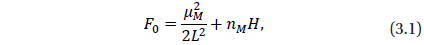
The Hamiltonian F of a lunar orbiter taking the nonuniform distribution of the lunar mass in consideration, can be written as
where
with, ψ=a/r,
where S=sin i, and C=cos i.
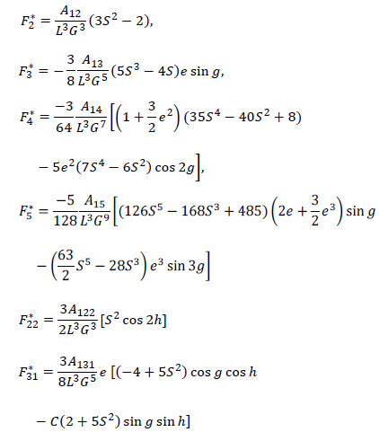
In order to study the motion of an orbiter a single-average is taken over the mean anomaly, l, of the orbiter. The average is defined as .
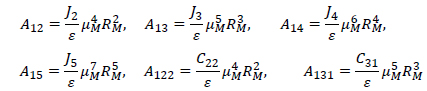
where, ε is the small parameter, and
with
and
To calculate the effects of C31 on IC , we will study two cases: First, we will study the combined effects coming from J2, and C22 on IC . Secondly, we will study J2 , C22 and C31 on IC .
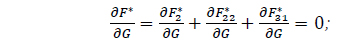
The critical inclination IC can be obtained from
which can be written as
where
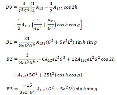
Let equation (7) be rewritten as
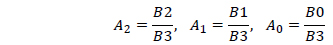
B0+B1x+B2x2+B3x3=0; x=cos i
The three roots of this cubic equation are given by
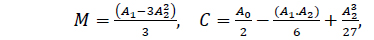
where
with
and
Depending on Equation (8); note that Equation (9) is neglected hence since it contain imaginary part, different simulations will be introduced here to distinguish the effect of C31 on lunar critical inclination IC with different ranges of a and e for both g and h being set to arbitrary constants in each case.
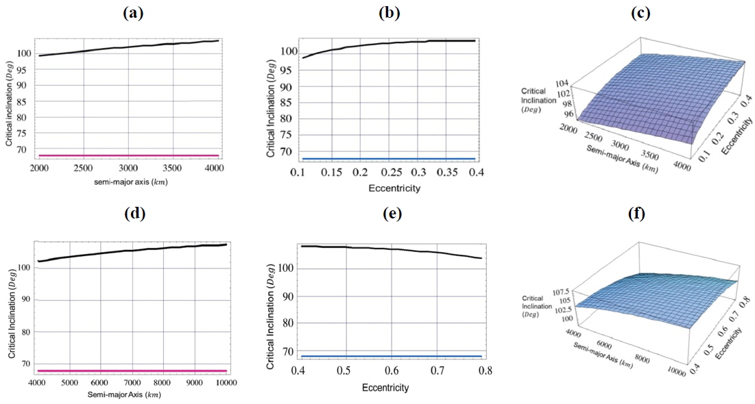
In all figures the black curves shows the critical inclination considering the effcts of J2, C22, and C31 while the red or blue ones represent the critical inclination IC considering just the effects J2 and C22, in two different cases as shown in the figures:
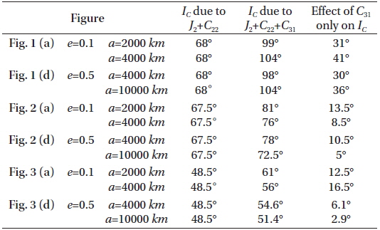
In the first case labeled by Figs. 1(a), 2(a), 3(a), we set the semi-major axis to the range 2000≤a≤4000 km and constant eccentricity e=0.1.
[Fig. 1.] Critical inclination as a function of, 1- semi-major axis (Fig. a, Fig. d) with eccentricity =0.1,0.5, 2-eccentricity (Fig. b, Fig. e) with semi-major axis =4000km,10000km, 3- both semi-major axis and eccentricity (Fig. c, Fig. f), argument of perigee ω=90°, and longitude of the ascending node Ω=270°.
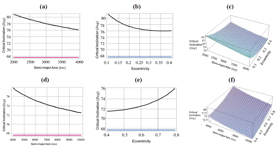
[Fig. 2.] Critical inclination as a function of, 1- semi-major axis (Fig. a, Fig. d) with eccentricity =0.1,0.5, 2-eccentricity(Fig. b, Fig. e) with semi-major axis =4000km,10000km, 3- both semi-major axis and eccentricity (Fig. c, Fig. f), argument of perigee ω=270°, and longitude of the ascending node Ω=270°.
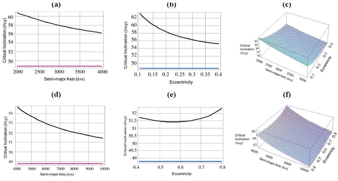
[Fig. 3.] Critical inclination as a function of, 1- semi-major axis (Fig. a, Fig. d) with eccentricity =0.1,0.5, 2-eccentricity(Fig. b, Fig. e) with semi-major axis =4000km,10000km, 3- both semi-major axis and eccentricity (Fig. c, Fig. f), argument of perigee ω=60°, and longitude of the ascending node Ω=18°.
In the second case labeled by Figs. 1(d), 2(d), 3(d), we set the semi-major axis to the range 4000≤a≤10000 km and constant eccentricity e=0.5.
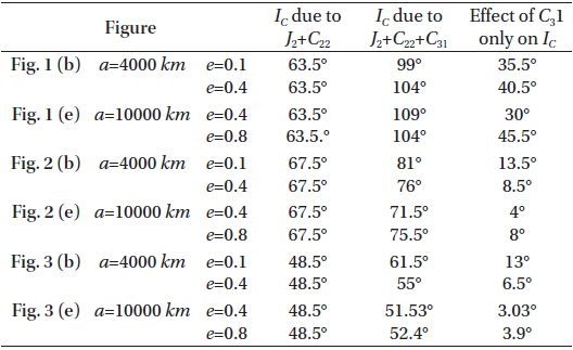
In the third case labeled by Figs. 1(b), 2(b), 3(b), we set the critical inclination versus the eccentricity 0.1≤e≤0.4 and the constant semi-major axis a=4000 km.
In the fourth case labeled by Figs. 1(e), 2(e), 3(e), we set the critical inclination versus the eccentricity 0.4≤e≤0.8 and the constant semi-major axis a=10000 km.
We repeat these case with different argument of perigee and longitude of the ascending node.
In Fig. 1:
taking account of the dynamical shape parameters J2 , C22 , and C31 , the critical inclination is plotted as function of the semi-major axis 2000≤a≤4000 km with constant eccentricity e=0.1. We obtained an increasing family of the critical inclinations ranging from IC≅99° to IC≅105°, for the corresponding semi-major axis, as seen by the black curve in Fig. 1 (a). Also we have a different increasing family of the critical inclinations ranging from IC≅98° to IC≅105° corresponding to eccentricity range of 0.1≤e≤0.4 with constant semi-major axis a=4000 km, as shown in Fig. 1 (b). Upon neglecting the effect of dynamical shape parameter C31 and considering only the combined effects J2 and C22 we have only one critical inclination angle of IC≅68°. This result reflects how big the effect of C31 on the critical inclination is. We can say that this parameter is responsible for the generation of the above mentioned families of critical inclinations. The same situations hold for curves in Fig.1 (d), We have plotted the critical inclination versus the semi-major axis 4000≤a≤10000 km with constant eccentricity e=0.5. We have obtained different increasing family of the critical inclinations ranging from IC≅102° to IC≅110° depending on the altitudes. While in Fig.1 (e), we have obtained different decreasing family of the critical inclinations ranging from IC≅110° to IC≅102° for corresponding critical inclination versus the eccentricity of 0.4≤e≤0.8 with constant semi-major axis a=10000 km. Again, C31 is the responsible parameter for the generation of these families of critical inclinations.
In Fig. 1 (c) and Fig. 1 (f), we plotted three dimensional figures of the critical inclinations versus the semi-major axis and the eccentricity for the values mentioned in Fig. 1 (a), Fig. 1 (b), Fig. 1(d) and Fig. 1 (e) respectively.
In Fig. 2:
taking account of the dynamical shape parameters J2 , C22 , C31 , the critical inclination is plotted as a function of the semi-major axis, 2000≤a≤4000 km with constant eccentricity e=0.1. We obtained a decreasing family of the critical inclinations ranging from IC≅81° to IC≅76°, for the corresponding semi-major axis, see the black curve in Fig. 2 (a). Also we have decreasing family of the critical inclinations ranging from IC≅82° to IC≅76° corresponding to eccentricity range of 0.1≤e≤0.4 with constant semi-major axis a=4000 km, as shown in Fig. 2 (b). Upon neglecting the effect of dynamical shape parameter C31 and considering only the combined effects J2 and C22 , we have only one critical inclination angle of IC≅67.5°. This result shows again how big the effect of C31 on the critical inclination is. It is also responsible for the generation of the above mentioned families of critical inclinations. The same situations hold for curves in Fig. 2 (d). We have plotted the critical inclination versus the semi-major axis 4000≤a≤10000 km with constant eccentricity e=0.5. We have obtained differently decreasing family of the critical inclinations ranging from IC≅77.7° to IC≅72.5° with different altitudes. While in Fig. 2 (e), we have obtained differently increasing family of the critical inclinations ranging from IC≅71.5° to IC≅76° for corresponding critical inclination versus the eccentricity of 0.4≤e≤0.8 with constant semi-major axis a=10000 km.
In the Fig. 2 (c) and Fig. 2 (f), we plotted three dimensional figures of the critical inclination versus the semi-major axis and the eccentricity for the values mentioned in Fig. 2 (a) and Fig. 2 (b), and Fig. 2 (d) and Fig. 2 (e), respectively.
In Fig. 3:
taking account of the dynamical shape parameters J2, C22, C31, the critical inclination is plotted as a function of the semi-major axis 2000≤a≤4000 km with constant eccentricity e=0.1. We obtained a decreasing family of the critical inclinations ranging from IC≅60.5° to IC≅56.5°, for the corresponding semi-major axis, as can be seen by the black curve in Fig. 3 (a). Also, we have a differently decreasing family of the critical inclinations ranging from IC≅63° to IC≅55.5° corresponding to eccentricity range of 0.1≤e≤0.4 with constant semi-major axis a=4000 km, as indicated in Fig. 3 (b). Upon neglecting the effect of dynamical shape parameter C31 and considering only the combined effects J2 and C22, we have only one critical inclination angle at IC≅48.5°. This result confirms again how big the effect of C31 on the critical inclination is. It is also responsible for the generation of the above mentioned families of critical inclinations. The same situations hold for curves in Fig. 3 (d). We have plotted the critical inclination versus the semi-major axis, 4000≤a≤10000 km, with constant eccentricity e=0.5. We have obtained differently decreasing family of the critical inclinations ranging from IC≅55° to IC≅51.5° according to these various altitudes. While in Fig. 3 (e), we have obtained two different families of the critical inclinations: the first family is decreasing ranging from IC≅51.8° to IC≅51.4° for corresponding eccentricity range of 0.4≤e≤0.55 and the second family is increasing ranging from IC≅51.4° to IC≅53° for corresponding eccentricity range of 0.55≤e≤0.8 with constant semi-major axis a=10000 km.
In Fig. 3 (c) and Fig. 3 (f), we plotted three dimensional figures of the critical inclination versus the semi-major axis and the eccentricity for the values mentioned in Fig. 3 (a), Fig. 3 (b), Fig. 3 (d) and Fig. 3 (e), respectively.
We can observe the following from the figures:
1) The orbital parameters especially the eccentricity and the semi-major axis do not affect so much the location of the critical inclination when we have considered only J2+C22, but when we consider J2+C22+C31, we have a number of families of critical inclinations as analyzed before. 2) Setting the argument of pericentre ω=90°, and the longitude of the ascending node Ω=270° yields one family of increasing critical inclinations. And we two families of decreasing critical inclinations when we set ω=270°, Ω=270°or ω=60°, Ω=18°, respectively. 3) The remarkable effect is that C31 is the responsible parameter for all these families of critical inclination.4) The reversed nature among some figures may be interpreted due to different selections of argument of pericentre. 5) For the same values of semi-major axes or the same eccentricities, we have different families of critical inclinations. These may be attributed to the passage of a satellite over different regions on the peculiar surface of the Moon with different mass distribution. It is quite clear from the result for the different choices of argument of pericentre and the longitude of the ascending node. 6) The slopes of all curves are not same which means the effects are of nonlinear nature.
Finally, we can collect our in the following Tables 1-2.
This study clearly shows the change in critical inclination values based on the investigation of the effect of the first tesseral harmonic coefficient, C31. The combined effect of the first zonal and sectorial parameters J2+C22 reveals that perturbing terms do not affect the critical inclination significantly. However, when we include the first tesseral harmonic coefficient C31, it was found that the critical inclination is strongly affected and we have different families of critical inclinations. These families may be used to design missions around the Moon with periodic orbits. It is observed that the variation of the argument of pericentre and the longitude of the ascending node affect the critical inclination so much. These effects may be attributed to the passage of a satellite over different regions on the peculiar surface of the Moon with different mass distribution. In the forthcoming work the authors aim to extend this work so as to include the effects of relevant higher harmonics of the Moon's gravitational field.