Mobile phones are viewed under various illumination levels. The displayed images on a mobile display can be perceived with a significant loss in contrast in daylight conditions. Image quality degradation in ambient lighting is mainly caused by screen reflections and light adaptation of the human visual system (HVS). Screen reflections decrease the contrast and color gamut of a mobile display by increasing the luminance of dark areas. Light adaptation of the HVS is another important factor. Images displayed in daylight are perceived as relatively dark due to light adaptation of the HVS because the luminance of a mobile display is considerably lower than that of the outdoor environment [1]. Moreover, the perceived image contrast changes according to different surround luminance levels [2]. CIECAM 97s [3] and CIECAM02 [4] color appearance models, developed by the Commission Internationale de L'Eclairage (CIE), determined the surround compensation ratios for average, dim, and dark levels. Various algorithms, such as illuminant adaptive color reproduction [1, 5] and veiling glare correction [6] for mobile displays, have been proposed to solve this image quality degradation problem. Display adaptive tone mapping operators can also be used to minimize visible contrast distortions for mobile displays [7]. All these works considered little about the spatial contrast discrimination ability of HVS in ambient lighting.
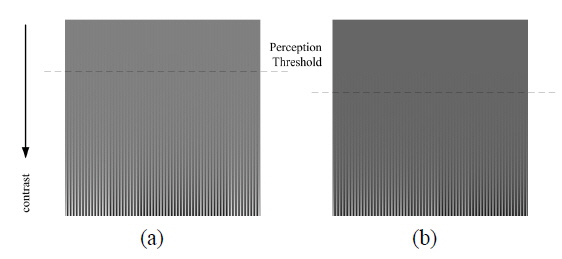
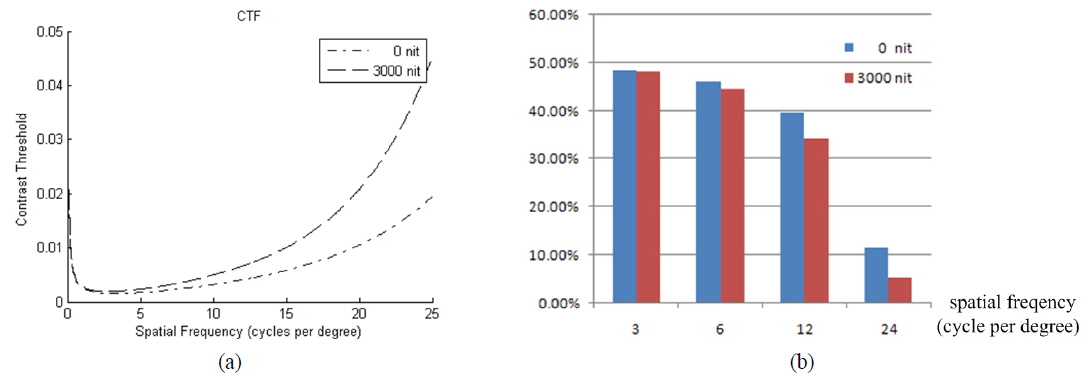
In recent work, Kim [8] examined the effects of surround luminance on the shape of the spatial luminance contrast sensitivity function (CSF), which represents the amount of minimum contrast at each spatial frequency that is necessary for a visual system to distinguish a sinusoidal grating or Gabor patterns over a range of spatial frequencies from a uniform field. In bright surrounding conditions, a large amount of reduction in contrast sensitivity at middle and high spatial frequencies can be observed; however, only a small amount is observed at low frequencies. As a result, a greater number of image details cannot be detected because the contrast perception threshold rises in ambient lighting, especially at middle and high frequencies. Figure 1 shows the degradation of contrast perception for a middle frequency sine wave image.
In later research [9] by Kim, a global image enhancement method is proposed to compensate the perception degradation. This method enhances whole spatial frequencies of the display image based on the degraded contrast sensitivity function with a frequency filter. Kim’s method implies that the contrast sensitivity function measured at various spatial frequencies can be implemented as a modulation transfer function of the system in the Fourier domain for image filtration.
Employing an image processing method to obtain the same perceived image for viewers is an attractive idea. However, the perceived contrast may vary greatly across the image because human contrast sensitivity varies with local average luminance [10]. Thus, the perceived contrast in complex image cannot be represented by a single value or different values in the spatial frequency domain. A number of “local band contrast” measure methods have been proposed for other image processing approaches. These definitions of contrast [10, 11] in these methods assign a contrast value to every point in the image for each spatial frequency band. Numerous applications have been identified for these definitions, especially in HVS-related image processing problems [12-14].
The objective of this paper is to enhance the local band contrast in images to compensate for perceived contrast degradation in ambient light. We proposed a perceived contrast compensation method based on local band contrast, which is extracted from the displayed image considering display factors. As our aim is not to mitigate the degradation in image quality caused by screen reflections in ambient lighting, our proposed method avoids changing other image properties, such as lightness and hue. Thus, it can be combined with other illuminant adaptive color reproduction and tone mapping methods.
II. HVS CONTRAST SENSITIVITY REDUCTION
The HVS is a nonlinear system with a very large dynamic range that behaves as a band-pass spatial filter [15]. The spatial filtering property is characterized by the CSF, which describes how contrast sensitivities vary as a function of spatial frequency. CSF exhibits a peak in contrast sensitivity at 4.0 ~ 5.0 cycles per degree (cpd) [16] and drops at both lower and higher frequencies. By measuring the minimum contrast at each spatial frequency in experiments, it has been deemed necessary for visual systems to distinguish a sinusoidal grating or a Gabor pattern over a range of spatial frequencies from a uniform field.
The CSF model used was originally proposed by Barten [17] as a function of spatial frequency and as dependent on field size (or viewing angle in degrees) and mean luminance of the sinusoidal grating stimulus. As the mean luminance of the sinusoidal grating stimulus decreases, the contrast sensitivity at each spatial frequency and maximum resolvable spatial frequency decrease. In addition, the shape of luminance CSF likewise changes: the peaks in the functions shift toward lower spatial frequencies, broaden, and eventually disappear [18, 19].
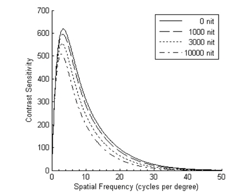
Kim identified characteristics of the HVS in the spatial frequency domain by considering surround luminance[8] as shown in Fig. 2. In general, the effect of surround luminance on the luminance CSF appears similar to that of mean luminance. A variable for compensating for surround luminance effect φ is multiplied with adaptive luminance L, as shown in Equation 1 [9].
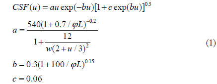
where

The surround luminance effect function φ forms a nonlinear function of luminance for approximating the perceived brightness reduction effect caused by increases in ambient illumination level. The surround luminance
where
According to the HVS model, an image detail can be detected if its contrast is greater than the threshold. Consequently, the amount of perceived contrast information changes with the contrast threshold level. Because ambient lighting affects the contrast threshold level of human vision, the same information for the image displayed at different ambient lighting levels cannot be perceived.
III. PERCEIVED CONTRAST COMPENSATION METHOD
An image stored as a matrix of pixel values is the most common representation for image processing; however, it does not reflect the way humans perceive images [20]. The response of the HVS depends much less on absolute luminance than on the relation of local variations to surrounding luminance. Meaningful visual information in images is mainly conveyed by contrast because the HVS has specialized cells that process signal contrast (rather than absolute signals) [20, 21]. The proposed method serves to compensate local contrast in images to improve image quality in ambient light.
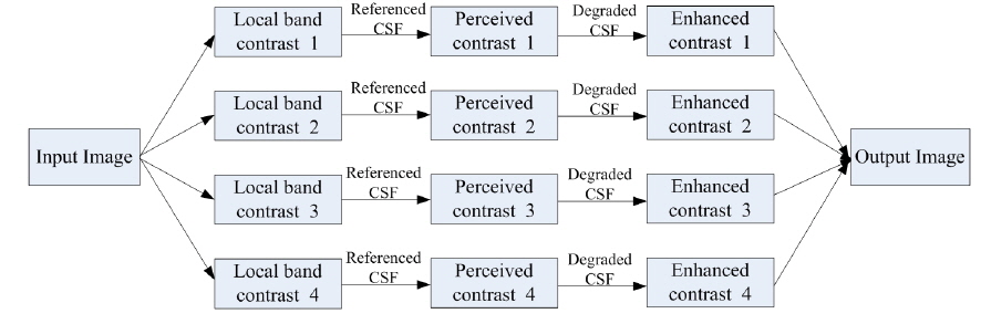
Perceived contrast may vary greatly across the image. To simulate nonlinear, threshold characteristics of spatial vision, several local band contrast definitions have been proposed [10, 11]. These definitions provide a method for transforming a pixel value image into several local band contrast images. Inspired by this research, we propose a perceptual contrast processing framework as depicted in Fig. 3.
In this method, the image is not directly enhanced; instead, the image is transformed into local band contrast data. Because these contrasts degrade under ambient illumination as described by the Kim CSF, our method enhances them to compensate the details and reconstruct the output image with these enhanced contrasts.
3.1. Local Band Contrast Computation
The contrast of simple patterns, such as the sinusoidal pattern or a square on a uniform background, is well defined as a single value, such as the Weber contrast and Michelson contrast; however, this is not true for real-world images. As mentioned earlier, perceived contrast may greatly vary across the image because human contrast sensitivity varies with local average luminance. Peli [10] proposed a complex contrast model in which the contrast of an image can be locally defined. Because human contrast sensitivity is highly dependent on spatial frequency, local contrast for each spatial frequency band is separately calculated. Lubin [22] modified Peli’s contrast for image quality metric, and Winkler [11] defined an isotropic contrast measure computed from an oriented filter. Since these definitions do not consider display factors, such as display black level and reflection light, thus resulting in contrast deviations in low luminance areas of images, we modify the local band contrast.
A mobile display is limited by maximum luminance and black luminance. The displayed luminance in ambient lighting can be modeled as Equation 4 [7]:

where
Using

Here,
For every band-pass filtered image

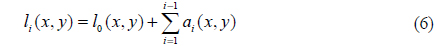
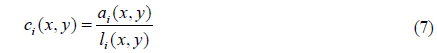
The local band contrast image is calculated as in Equation 7:
3.2. Perceived Contrast Compensation in Different Band Contrast Images
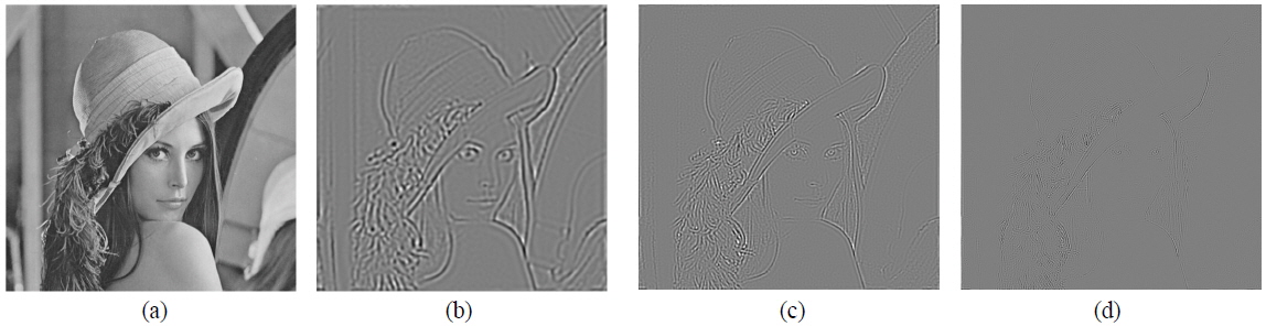
The amount of perceived contrast information changes with the threshold contrast level. In Fig. 4, fewer contrast details can be perceived in the high frequency contrast images (Fig. 4(c) and (d)) compared to the low frequency contrast images (Fig. 4(b)) because a larger number of contrast values in the high-frequency contrast images are lower than the threshold.
Further, because ambient lighting affects the contrast threshold level of human vision, the same information for the image displayed at different ambient lighting levels cannot be perceived. For example, assuming that the surround luminance is 3000 cd/m2, a greater number of details is below the threshold and fewer are perceived, as shown in Fig. 5. Most contrast information is lost in the middle frequency, while only a small amount of information is lost in the low and high frequencies.
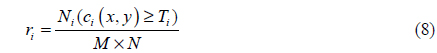
The ratios of different band contrast details are calculated as in Equation 8.

where
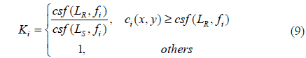
To compensate for the loss in image contrast caused by an increase in surround luminance, the compensation ratio in different bands should be confirmed. These compensation ratios of different bands are determined by the contrast threshold difference between the reference (dark level) and given target surround luminance. In each contrast image, the contrast value above the threshold should be amplified by the matching ratio; those below the threshold are not processed to prevent noise amplification because human vision cannot detect them even in an environment without ambient lighting.

where
Note that contrast masking is not involved when counting compensation rate for different frequency band here. Contrast masking [23] typically involves an increase in the HVS contrast threshold for a signal in the presence of another one. Some contrast information above the contrast threshold may be undetectable for the contrast masking phenomenon. In contrast perception evaluation, ignoring the contrast masking effect will result in an excessive contrast estimate. However, in the compensation method, the contrast masking phenomenon exists in both the original and the output image, because of which their effects are counteracted to some extent. Contrast masking is hence not involved in our proposed method.
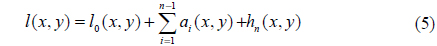
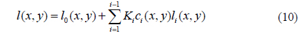
Finally, the output image is reconstructed in incremental steps by these enhanced contrast images. The reconstruction must be a low frequency to high frequency progression because
The aim of our proposed approach is to compensate for all contrast details to match those in an ideal environment without changing other image characteristics. We therefore designed an experiment to test contrast detail visibility in different environments.
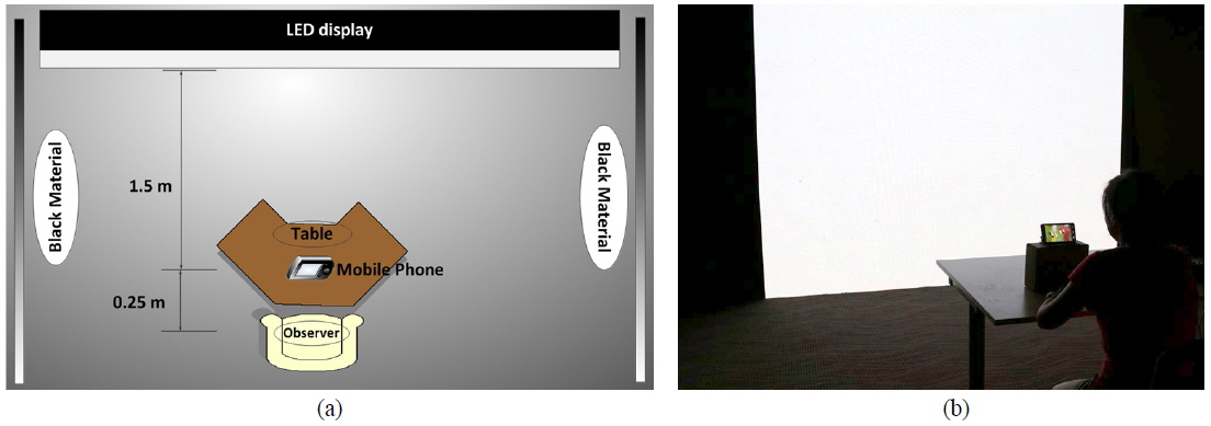
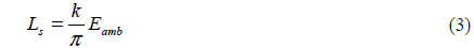
A darkroom with a large LED display was selected as the test environment (Fig. 6). This display was designed with surround lighting for which the brightness could be automatically adjusted, and the color temperature was approximate to D65. A mobile phone was placed in front of the LED display and the same orientation was maintained. This ensured that the background brightness could be accurately controlled when viewing the mobile phone. The LED display was secured as the only light source in the darkroom; therefore, light reflected on the mobile phone screen would be controlled at a low level.
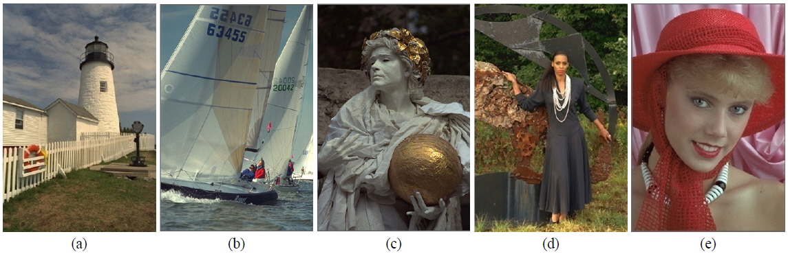
Five test images were selected from the LIVE Image Quality Assessment Database [24]. The images were of a lighthouse, a sailing boat, a statue, a standing woman and a woman in a hat as shown in Fig. 7. Because our method only enhanced the contrast extracted from the gray image, these RGB images should be converted into the HSV. Only brightness was applied through the enhancement procedure; chrominance properties were preserved.
The test comprised two stages, one in the darkroom environment and the other in a high ambient light environment, controlled by LED display adjusted in 3000 cd/m2 as the surround luminance. In the darkroom, the five images were tested. In the high ambient light environment, the five images were enhanced by Kim’s method and our proposed method. As a result, a total of 15 test images, including five original ones and 10 enhanced ones, were randomly displayed for testing in the high ambient light environment.
In both stages, observers sat in front of the display and gradually adapted to the ambient light. The 4.7-in mobile phone—placed at a fixed distance of 25 cm—randomly displayed each image. All images were randomly display for two rounds. In the first round, observers just browsed all images and were told to notice “detail visibility” of each image. In the second round, they were asked to score each image by assessing the level of “detail visibility”. The score was a 5-rating scale, from “hardly visible” (1) to “the most visible” (5).
Nine observers (five male and four female) with normal color vision were selected as subjects for our experiment. The experimental results, average scores for each test image, are provided in Table 1. The detail visibility of images processed by our proposed method are higher than that of the original images in the ambient light and enhanced by Kim’s method, and nearly equal to that in a dark room.
[TABLE 1.] Five levels of detail visibility
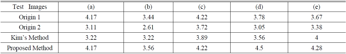
Five levels of detail visibility
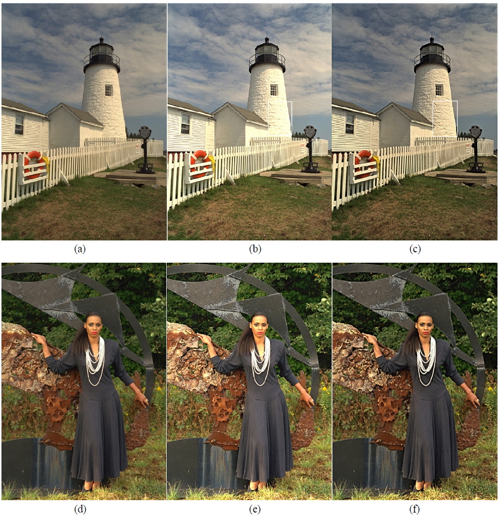
In Fig. 8, two test images enhanced by Kim’s method and the proposed method are presented. In both methods, the contrast of details has significantly improved, as shown by the cloud and grass in Fig. 8(b) and 8(c), the rock and leaves in Fig. 8(e) and 8(f). Kim’s method globally enhanced all frequencies in the Fourier domain, including the direct current component, with consideration of the contrast masking. As a result, we can observe higher brightness and the loss of contrast details in the highlighted region (as shown by the lighthouse in Fig. 8(b)).
In the proposed approach, only local band contrast is extracted from original image and adjusted, so other image characteristics, such as lightness and hue, are maintained. On the other hand, as the compensation ratios for each of the local band contrasts are strictly deduced by the CSF degradation value as Equation 9, an over-enhancement problem can be avoided. So this approach can enhance the contrast of images without changing other image characteristics.
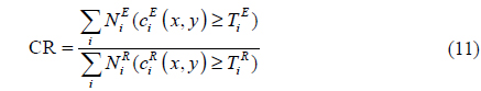
Limited research has been conducted on the influence of viewing conditions in objective visual quality metrics; moreover, the issues relating to ambient illumination have been largely unexplored [25]. Here, we use a ratio of perceived contrast amounts in ambient lighting to those in an ideal environment to evaluate the compensation effect. We sum all pixels in different contrast bands to determine the perceived contrast ratio (CR) as Equation 11:

where is the pixel number of which the contrast value is larger than threshold in band i enhanced contrast is that in . The sum of reflects the perceived contrast amount in ambient lighting and that of reflects the amount in a reference environment.
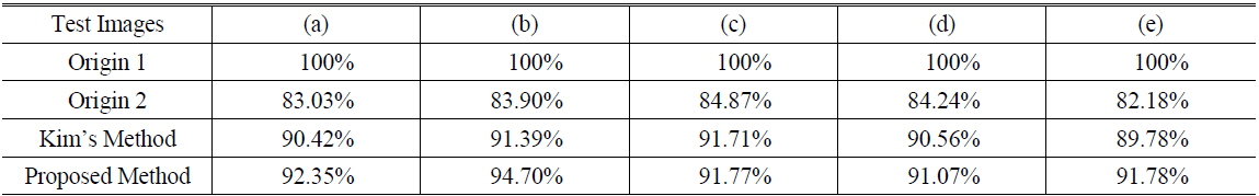
In Table 2, perceived contrast ratios of the origin image in ambient light are quite small, for many contrast details are lost. In both Kim’s method and the proposed method, the contrast ratios become larger as contrasts increase; however, they nevertheless do not reach 100% of Origin1 because the contrast gains are limited by the dynamic range of the image.
[TABLE 2.] Perceived contrast ratios in five images

Perceived contrast ratios in five images
The dynamic range is a limitation of this contrast compensation method. Because all band contrast images are enhanced by a factor greater than 1.0, the range of final compensation images—the sum of all band images—is typically greater than the original range of gray levels. Therefore, the final image does not provide sufficient enhancement at different frequencies, especially at the high frequency. Fortunately, as the output image is reconstructed from low frequency band contrast to a high frequency one, in most cases only the highest frequency band contrast, which contains less detail than other bands, is limited by dynamic range. In Kim’s method, all frequencies are enhanced with consideration of the contrast masking, which results in more gray values exceeding the dynamic range of the image and smaller contrast perceived ratios as in Table 2.
In this paper, we proposed a perceived contrast compensation method that processes the extracted local band contrast from the original image. Experimental results demonstrated that this method can effectively enhance contrast details without changing other image characteristics; moreover, most contrast details can be compensated even in high ambient illumination. Although the image dynamic range may be a limitation of our method, only a small number of contrast details are limited by it.