Since the early of 20th century, many designs have been suggested with the intention of widening a camera’s field of view. Fisheye lenses and omni-directional optical systems are among the proposed designs. A fisheye lens system was first proposed by Robert W. Wood at 1911 in the book of
The omni-directional optical system was first proposed by Rees in 1970 in a United States Patent that would use a hyperbolic mirror to capture images [3]. An omni-directional camera has a horizontal field of view of 360 degree and a wide field in the vertical plane as well. It has already been adopted for many applications, including security, surveillance, visual navigation, tracking, localization, teleconferencing, and camera-networking [4]. For the omni-directional optical system, two main methods have been proposed: 1) a mechanical approach, and 2) an optical approach. The mechanical approach uses several lenses in the horizontal direction or rotates the lenses to obtain a 360-degree horizontal field of view. This method is a straightforward but also has a drawback of real-time imaging and alignment among the multiple lenses [5]. Another method in optical approach is a catadioptric system, which uses parabolic, hyperbolic, or elliptical mirrors. However, only donut-shaped images can be obtained since the catadioptric system has central obscuration due to its use of multiple mirrors.
The goal of both omni-directional and fisheye lens systems is to obtain a panoramic field of view, but each system has only a fixed field of view and cannot incorporate the other system’s advantages, so each has a limited usage range. In the case of an optical system that could obtain not only a 360-degree field of view horizontally, but also a 180-degree field of view along the front angle by changing the field of view for each purpose, we would expect a wider range of use because a varifocal system has multi-configuration of view field [6, 7]. For example, the user could take a picture of a wide landscape in front of the optical system with a fisheye lens configuration. In the case of shooting surrounding scenery like panoramic photos, an omni-directional configuration can capture a 360-degree image in the horizontal direction. Each configuration can be converted easily, if necessary.
2.1. Distortion Mapping and Design Concept
Distortion is a decisive factor to determine the field of view in an optical system with a wide field of view. If we suppose that the field of view is related to only Y = f·tan
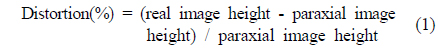
In other words, we can obtain an optical system with finite image height even though it has a field of view of more than 180 degrees due to distortion.
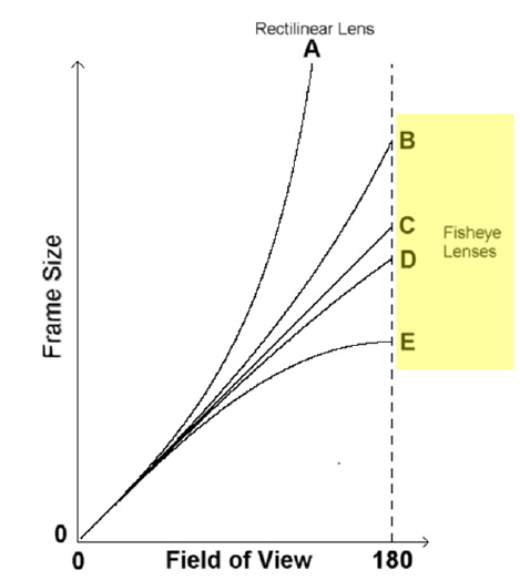
In an optical system with a field of view of 180 degrees or more, we can obtain a relationship between distortion and image height by using the distortion mapping. There are four kinds of mapping functions, as shown in Table 1. We can calculate the field of view and image height with each mapping function. In the case of a fisheye lens, which has a 180-degree field of view, we can obtain the graph shown in Fig. 1 [9]. In the graph for the case of an optical system that obeys Y = f·tan
[TABLE 1.] Distortion mapping function

Distortion mapping function
The most common mapping functions are the equidistance and equisolid-angle types. We applied the equisolid-angle mapping function to design the omni-directional fisheye varifocal lens system. For this purpose, it is necessary to decide the FOV (field of view) and IH (image height) in advance. Based on the calculation results, we can determine the respective focal lengths for the omni-directional configuration and the fisheye configuration, separately.
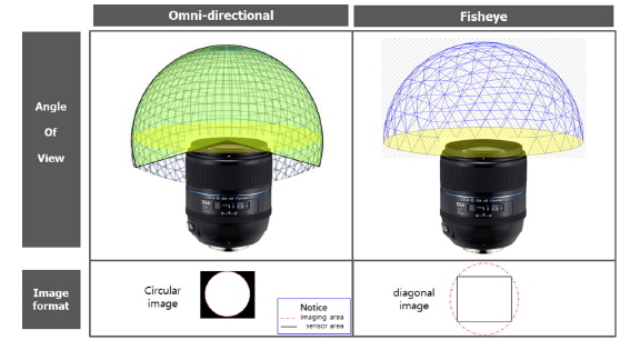
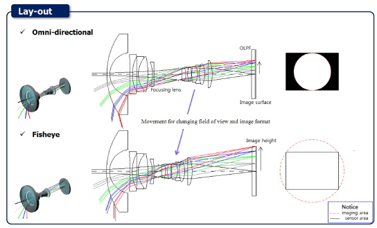
We want to describe the concept of the omni-directional fisheye varifocal optical system. Even though the newly-proposed system combines the existing fisheye and omni-directional optical systems, it has a broader range of use and can solve the drawbacks of catadioptric omni-directional systems. A conventional catadioptric system has multiple reflective surfaces to obtain an image of the direction orthogonal to the optical axis. Instead, we suggest a system like that shown in Fig. 2, which has a FOV of more than 180 degrees without reflective surfaces so it can form an the image of the direction orthogonal to the optical axis. Therefore, it is possible to obtain a 360-degree horizontal image, as well as a complete front image, whereas a conventional catadioptric system has central obscuration due to its mirrors. Furthermore, we can reduce the manufacturing difficulties in the mirror system.
To realize the proposed design, we made a full frame type of fisheye configuration with a 180-degree field of view diagonally across a square sensor, and a circular type of omni-directional configuration with a 210-degree field of view vertically across a square sensor. There are notable differences between the fisheye configuration and the omni-directional configuration in terms of image format. The fisheye configuration has a rectangular image while the omni-directional configuration has a circular image. We will generate rectangular images in fisheye configuration because a full frame type imaging is the most common and efficient method when using a full sensor. In contrast, we will create circular images in omni-directional configuration because we can obtain a 360-degree field of view orthogonally to the optical axis for the image rectification [10]. The image format and field of view are shown in Fig. 2.
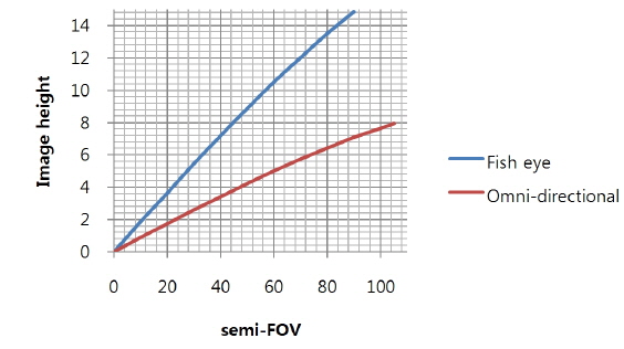
Using the mapping function of equisolid angle type, we can get the result of calculation that can show the relationship between image height and field of view, as shown in Fig. 3 and Table 2. In addition, the design specifications are summarized in Table 2.
[TABLE 2.] Design specification
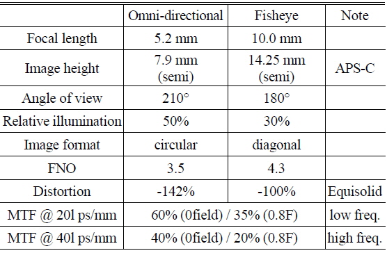
Design specification
The omni-directional and fisheye varifocal system is shown in Fig. 4, based on the design points mentioned above. It is composed of 12 spherical lenses, and divided into two main groups: a front group and a rear group. The front group has strong negative power for wide field of view from 180 to 210 degrees. Field of view more than 180 degrees enables the system to obtain a 360-degree image of the direction orthogonal to the optical axis. In contrast, the rear group has positive power. When the rear group moves toward the object side while changing focal length, the field of view and image size (format) are changed. The fisheye configuration has a 180-degree FOV and produces a full frame type image. On the other hand, the omni-directional configuration has a 210-degree FOV and produces a circular type image. A 210-degree FOV and circular image type are necessary for a 360-degree image of the direction orthogonal to the optical axis.
Furthermore, the front group (negative power) is fixed, while the rear group (positive power) moves towards the object side to change the field of view. To adjust the position of the image surface according to the object distance (auto focusing) the last lens in the front group moves towards the front or the rear.
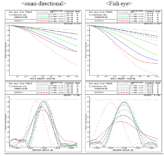
In optical performance criteria such as MTF, the results meet all design requirements. In particular, the omni-directional configuration demonstrates better optical performance than does the fisheye configuration, since the full field (the highest image height) matches the vertical image in the omni-directional configuration. The full field of the omni-directional configuration is necessary to have better performance than the fisheye configuration does.
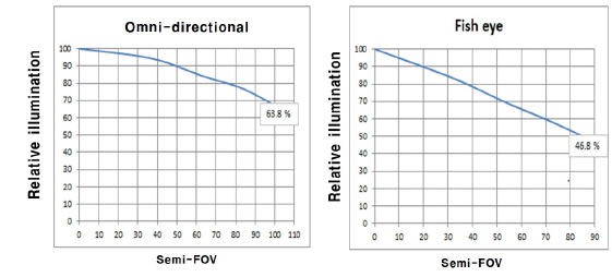
Relative illumination of the omnidirectional configuration also must be higher than for the fisheye configuration, since the full field of the omni-directional configuration matches the vertical field of the image after image rectification. Thus, we required the relative illumination to be more than 50 percent at the omnidirectional configuration. The actual design resulted in the relative illumination of 63.8 percent at omni-directional configuration and the relative illumination of 46.8 percent at fisheye configuration. In addition, the slope of the relative illumination graph is important for manufacturing. Our graph shows a gentle slope, demonstrating that we can prevent rapid decrease of illumination at the edges of the image.
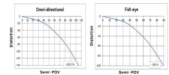
Figure 7 shows the same distortion as was previously calculated from the distortion mapping function.
Based on the actual design results, it is confirmed that our design achieved all required specifications including field of view, resolution, relative illumination and distortion.
3.1. Zernike Polynomial Coefficients
The MTF (Module Transfer Function) and wavefront error are the main optical performance evaluation parameters. MTF is the most common performance indicator in optical design, so we have extensive data and experience for MTF criteria. Unfortunately, MTF cannot be used in sensitivity analysis. Sensitivity analysis is the study of how performance changes due to inconsistencies in the manufacturing process (such as radius, thickness, tilt, decenter, etc.). Thus, sensitivity is a way to predict the actual product performance. However, MTF is not linearly related to sensitivity. This is why we cannot use MTF as a sensitivity parameter. Instead, wavefront error is the most useful parameter for sensitivity analysis [11]. The amount of wavefront error can be represented by PV (Peak to Valley) and RMS (Root Mean Square). It can also be represented by Zernike polynomials. Radial polynomials are combined with sines and cosines rather than with a complex exponential. The final Zernike polynomial series for the wavefront OPD, ΔW can be written as eq. (2) [12].
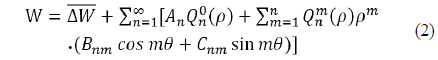
where is the mean wavefront OPD, and An, Bnm, and Cnm are individual polynomial coefficients. For a symmetrical optical system, the wave aberrations are symmetrical about the tangential plane and only even functions of
[TABLE 3.] Zernike polynomials and RMS wavefront conversion ratio [12, 13]
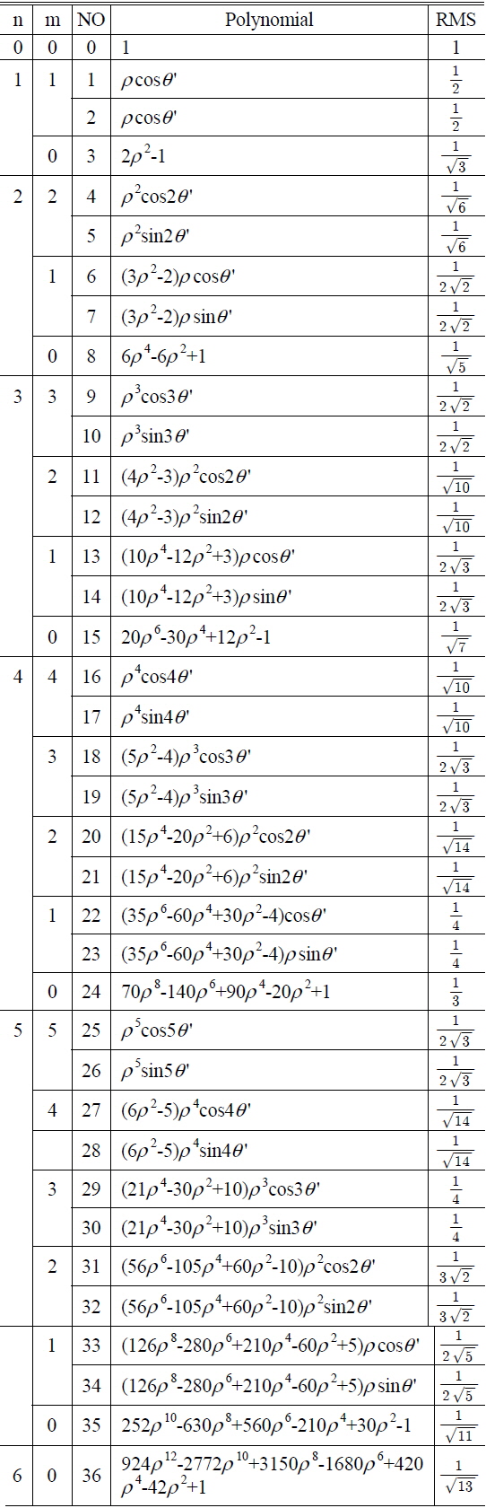
Zernike polynomials and RMS wavefront conversion ratio [12, 13]
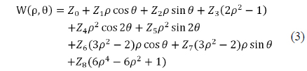
The first-order wavefront properties and third-order wavefront aberration coefficients can be obtained from the Zernike polynomials coefficients. Using the first nine Zernike terms, Z0 to Z8, as shown in Table 4, the wavefront can be written as eq. (3) [12].
[TABLE 4.] Aberration corresponding to the first nine Zernike terms [11, 12]
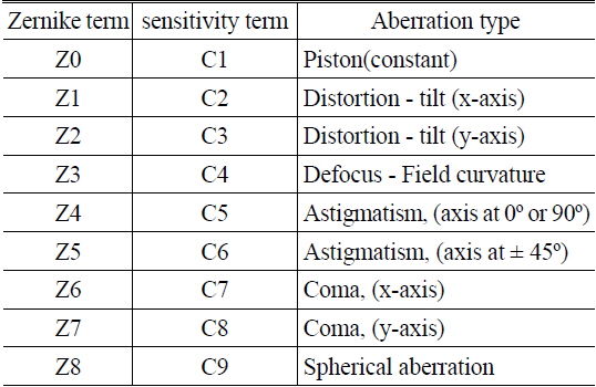
Aberration corresponding to the first nine Zernike terms [11, 12]
Zernike coefficients are linearly related to small manufacturing errors [11]. Using this property, we can define the sensitivity coefficient. The Zernike coefficient displacement ΔCi for a small displacement (error) ΔLj can be represented as eq. (4) [11]

where sensitivity Sij is .
If we calculate the sensitivity for all kinds of displacement based on the Zernike coefficients, we can obtain the total Zernike coefficient displacement, ΔCi, when random displacements arise. The various manufacturing errors can be divided into two major categories: symmetric error and asymmetric error. Symmetric error is caused by variations in symmetrical factors such as radius, thickness and index and results in changes in performance. Symmetric error causes the Zernike coefficients c4 (defocus) and c9 (spherical aberration) at 0field but it causes c4 (defocus), c5 (astigmatism), c8 (coma), c9 (spherical aberration) at 0.8field. In contrast, asymmetric error occurs due to asymmetrical factors, such as tilt and decenter. It generates the Zernike coefficient c5 (astigmatism) and c8 (coma), as well as c4 (defocus) and c9 (spherical aberration) at 0field and 0.8field. In this study, we use coefficients c4 through c9, which affect the image quality. The piston coefficient (c1) can be eliminated easily with proper control, and the distortion coefficient (c2, c3) do not affect the image quality. Further, coefficients higher than c10 are insignificant [11]. Consequently we use Zernike coefficients c4~c9 to analyze the wavefront aberration. The correspondence between Zernike coefficient terms and aberrations is shown in Table 4.
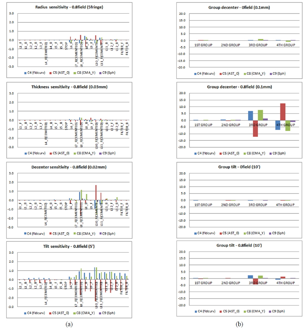
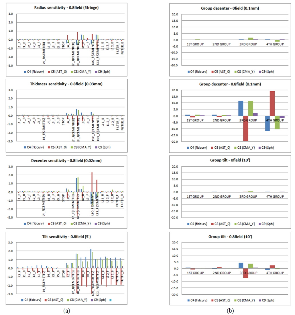
If we apply sensitivity analysis on the omni-directional and fisheye varifocal system, we can obtain the sensitivity graphs shown in Fig. 8 and 9. In the graphs, L1 denotes the first lens from the object side and L12 denotes the 12th lens from the object side. F and B next to the lens number signify the front and back surfaces of each lens. Sequentially from lens L1 to L12, we determined the manufacturing errors in radius, thickness, index, decenter, and tilt for each lens surface and calculated c4, c5, c8, and c9 displacements corresponding to these errors. c6 and c7 are excluded because displacement is zero in the y axis. Sensitivity was calculated separately 0field and 0.8field. In symmetric terms, we found that c5 and c8 are not generated in 0field. At the same time, we also determined that the radius sensitivity of L1B was not significant, even though the radius was so small that the lens was similar to a hemisphere. However, the radius sensitivity for L6 through L12 in the rear lens group was larger than in the front group. This same phenomenon appeared in the thickness and index. Furthermore we discovered that the rear lens group was more sensitive than the front group to asymmetric manufacturing errors, such as decenter and tilt. And sensitivity of 0.8field of view is much more sensitive than 0field. In 0.8field, decenter and tilt are the most sensitive error factors. Overall, the fisheye configuration is more sensitive than the omni-directional configuration. Figures 8 and 9 below show the sensitivity based upon the displacement of Zernike coefficients corresponding to manufacturing errors, for both the omni-directional and fisheye configurations.
In this section, we will analyze image quality degradation, based on the sensitivities mentioned in Section 3.2. First, we can examine errors caused by production. There are two kinds of manufacturing errors: unit part production error and assembly error. Unit part production error includes radius, thickness, index, and centering errors. Assembly error includes seat tilt, clearance, group decenter, and group tilt errors. We need to meet an error budget in all of these cases. We set a strict tolerance for the rear group due to high sensitivity.
For the actual production, we separated the front group into a 1st group and a 2nd group. In same way, we divided the rear group into a 3rd and a 4th group. We calculated the Zernike coefficient displacement and tolerance for every unit part and group. We assigned strict tolerances of 0.03mm for decenter and 5’ for tilt to the 3rd and 4th groups due to their high sensitivity. Close inspection of Fig. 8 and 9 shows that the fisheye configuration is more sensitive than the omni-directional configuration. We also found that the displacement direction of the Zernike coefficient caused by group decenter error is reversed between the 3rd and 4th groups. That means the Zernike coefficients will cancel out when the 3rd and 4th groups have the same direction of decenter. Thus, alignment between the 3rd and 4th groups is an important factor in maintaining the designed performance, since it allows for correction of image quality degradation using decenter compensation between the 3rd and 4th groups. We will discuss alignment and compensation in Section 3.4.
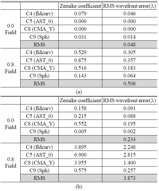
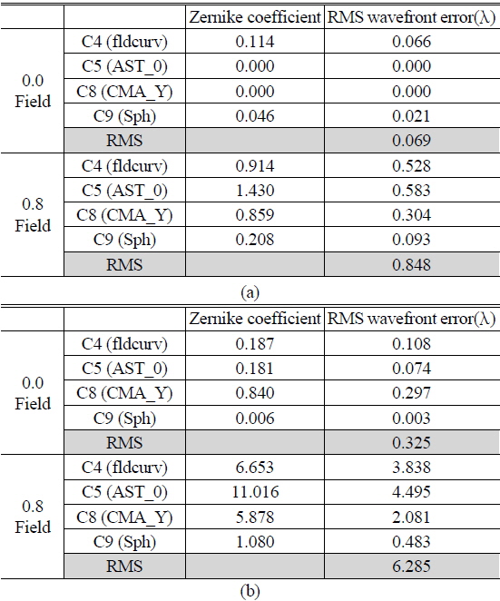
Displacement of the Zernike coefficients according to various error factors and given tolerances can be calculated to RMS (Root Mean Square). In the worst case, the displacement value of each surface could be the sum of absolute values. However, we have to use RMS instead of a simple sum since there are many cases in which the direction of displacement cancels out. Thus, we calculated the RMS value of every surface, which is converted from the Zernike coefficient. In evaluation of the optical system, RMS wavefront error and MTF (Module Transfer Function) are essential to image quality interpretation. Even though we can use RMS wavefront error, it does not have a sign such as “+” or “−”. MTF is not also appropriate for sensitivity analysis because of non-linearity. In the end, we must use Zernike coefficients, which have both sign and linearity. The Zernike coefficient can then be translated to RMS wavefront error. If the wavefront aberration can be expressed in terms of Zernike polynomials, then the RMS wavefront can be calculated simply based upon the orthogonality relations of the Zernike polynomials. The Zernike coefficient can be equivalent to RMS wave front error, as shown in Table 3 [12, 13]. We calculated Zernike coefficient displacement and RMS value for both symmetric and asymmetric error cases. Table 5 and 6 show the Zernike coefficient and RMS wavefront error calculation result.

Calculation result of Zernike coefficient & RMS wavefront error at omni-directional configuration (a) Symmetric error factors, (b) Asymmetric error factors

Calculation result of Zernike coefficient & RMS wavefront error at fisheye configuration (a) Symmetric error factors, (b) Asymmetric error factors
Table 5 and 6 reveal that the fisheye configuration has more RMS wavefront error, due to its higher sensitivity. Among symmetric errors, degradation of image quality is not significant. On the contrary, degradation of 0.8field is large. We expect that the omni-directional configuration has 3.873 λrms wavefront error variance in 0.8field and fisheye configuration has 6.285 λrms wavefront error variance in 0.8field.
3.4. Alignment and Compensation
In this section, we will discuss compensation for image quality degradation. To improve image quality, we need movement of lens. There are two kinds of movements: longitudinal movement and transverse movement for compensation. Longitudinal movement compensates symmetric error on axis such as defocus and spherical aberration and field curvature. Transverse movement of lens compensates off-axis asymmetric error such as coma and astigmatism. In this system, asymmetric sensitivity is overwhelming. Thus we need a compensation method to cancel out the asymmetric sensitivity using transverse movement of one of the lenses. There are several conditions for use of transverse movement compensation. First, it is necessary to be low sensitivity for 0field for compensation of 0.8field. Second, direction of sensitivity must be opposite that of error terms. Opposite direction of sensitivity means that same direction of movement can compensate other errors. Third, the amount of sensitivity is needed to be affordable for control by mechanical system. We have identified the most sensitive factor is decentering for each surface and group. However, we must note the direction of the Zernike coefficient according to the decentering. In particular, the 3rd and 4th lens groups are sensitive, but the signs of their Zernike coefficients are opposite, and the absolute value is similar for both the 3rd and 4th groups. In other words, the high sensitivities cancel since the sign of sensitivity is reversed and the absolute value is almost the same between 3rd and 4th groups. Thus, alignment between 3rd and 4th groups is essential and can affect both degradation and compensation of image quality. We chose the 3rd lens group as a compensator because it meets all conditions we mentioned above. Each group’s decenter and tilt sensitivity is shown in Table 7.
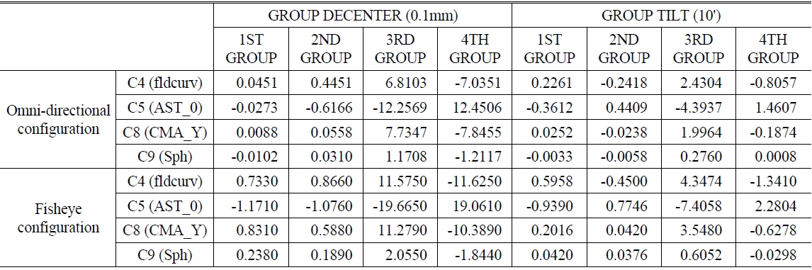
Zernike coefficients displacement from lens group decenter and tilt at 0.8 field (sensitivity)
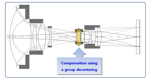
For a compensation system, we developed the mechanical design shown in Fig. 10, and suggest compensation system by using 3rd group decentering.
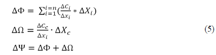
The final degradation amount is the sum of manufacturing error and compensation. Residual degradation amount can be described as shown eq. (5).

Where

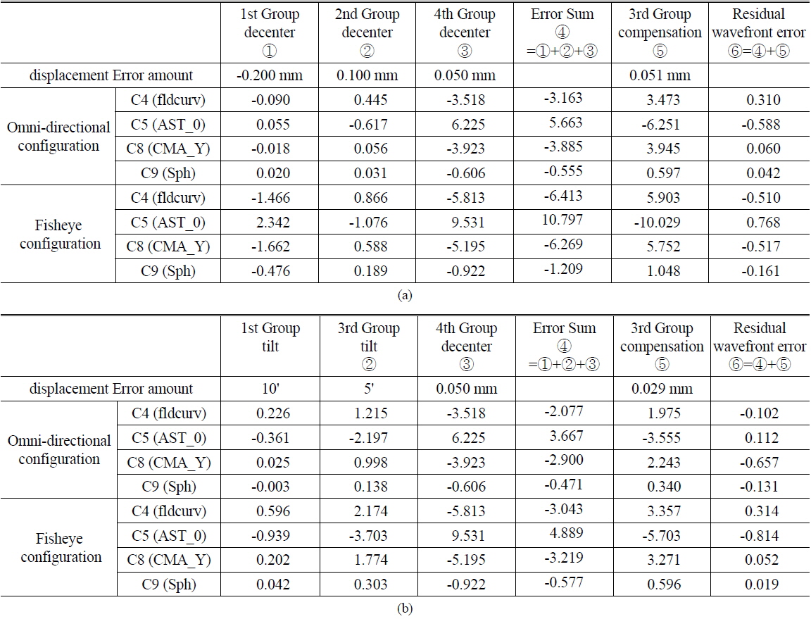
We note the sum of manufacturing errors and compensation result in Table 8. The 1st to 4th lens groups have manufacturing errors. The sum of each Zernike coefficients displacement is the degradation amount in image quality. Thus we need to decrease the sum of each Zernike coefficients displacement from manufacturing error. To minimize degradation of image quality, we can make intentional compensator displacement. Eventually, the total sum of Zernike coefficients displacement from both manufacturing error and compensator must be minimized. We could not show all kinds of cases, so we selected the two worst cases. In Case 1, this system has 1st group −0.2mm decenter, 2nd group 0.1mm decenter and 4th group 0.05mm decenter among group alignment. But if we compensate misalignment using the 3rd group decentering, MTF peak balance of 0.8-field is narrowed to match the design level. In Case 2, the system has 1st group 10’ tilt, 3rd group 5’ tilt, and 4th group 0.05 mm decenter simultaneously in group alignment. In Case 2, we considered the case of 3rd group tilt and 4th group decenter error case rather than 2nd group tilt and 4th group tilt because of higher sensitivity. However, the compensation system sufficiently corrects these errors in Case 2.
[TABLE 8.] Compensation calculation. (0.8field) (a) Case 1, (b) Case 2

Compensation calculation. (0.8field) (a) Case 1, (b) Case 2
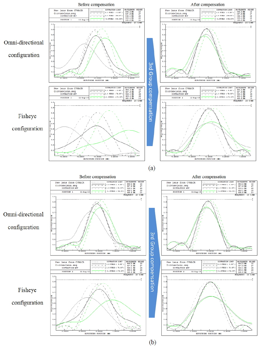
Furthermore we verified the compensation method through simulations. Through focus MTF shows peak balance of 0.8field at each edge. Figure 11 shows compensation result as MTF peak balance. We can recognize the effectiveness of tolerance analysis and compensation schemes in Table 8 and Fig. 11. In Table 8, we calculated the sum of Zernike coefficients from both manufacturing error and compensator. Thus we obtained solution of the minimum degradation. We confirmed above calculation as shown in Fig. 11. Compensation scheme works well as shown in through focus MTF peak balance.
In the study, we proposed a new optical system of omni-directional and fisheye varifocal lenses. Furthermore, we analyzed the sensitivity using wavefront error and established a compensation scheme for difficulties that may arise during manufacturing.
The new optical system has two different fields of view, which correspond to the fisheye and omni-directional configurations. The fisheye configuration has a 180-degree field of view and the omni-directional configuration has a field of view more than 180 degrees, so it can create an image direction orthogonal to the optical axis. If we get an image from direction orthogonal to the optical axis, it is possible to take 360 degrees images. This system does not include reflective surfaces to realize the omni-directional and fisheye varifocal lens, thereby eliminating central obscuration. It is also composed of a strong negative front group and a positive rear group.
The study results demonstrate that the system is able to satisfy the required specifications. However, we also needed to examine potential manufacturing difficulties, since there have been no similar system previously. Consequently, we performed a sensitivity analysis and studied compensation schemes using Zernike polynomial coefficients to determine effective corrections for manufacturing inconsistencies. To that end, we programed macro in CODE V® that can produce the sensitivity coefficient corresponding to a small manufacturing error. Furthermore, we calculated the sensitivity and tolerance of making unit part and assembling parts based on wavefront sensitivity. Finally, we established a method of optical axis alignment and compensation logic. We anticipate this paper gives good guidance for the optical design and tolerance analysis including compensation method in the extremely wide angle system.


![Graph of relationship between the field of view and frame size for a given focal length lens [9].](http://oak.go.kr/repository/journal/16136/E1OSAB_2014_v18n6_720_f001.jpg)


![Zernike polynomials and RMS wavefront conversion ratio [12, 13]](http://oak.go.kr/repository/journal/16136/E1OSAB_2014_v18n6_720_t003.jpg)
![Aberration corresponding to the first nine Zernike terms [11, 12]](http://oak.go.kr/repository/journal/16136/E1OSAB_2014_v18n6_720_t004.jpg)