In computer vision, multi-camera measurement systems have been widely utilized in various areas [1, 2], e.g., the 3D measurement, object reconstruction, object detecting and tracking, etc. Cameras in the multi-camera measurement system are fixed; therefore, the relationship between each pair of cameras is constant. One simple but typical kind of multi-camera measurement system is the stereo measurement system, which consists of two cameras with a common field of view. Based on the point pairs, the information about the point in the scene can be obtained from many limitations, such as epipolar constraint, etc. As a well-developed theory, the stereo measurement system has been widely utilized in many industrial areas. On the other hand, the cameras in the multi-camera measurement system are not always with a common field of view according to different tasks. Therefore, when the cameras in the system have no common field of view, it is called a non-overlapping multiple vision system. Although the non-overlapping multiple vision system has no common field of view, the range of the measurement is larger. The most important task is the calibration of cameras in the multicamera measurement system, i.e. obtaining the relationship between each two cameras.
The approaches to obtaining the relationship between cameras, which is called the calibration of the external parameters of the system, are various. These approaches can be classified into two categories according to the target which is used: one uses the exact coordinates of the feature points while the other relies on the geometric or algebraic properties.
In [3], M. Knorr presented an approach to calibrate the extrinsic parameters of a multi-camera system using a ground plane, from which the homographies can be deduced. As a natural reference object, the ground plane can be estimated using a single iterated extended Kalman filters. Obviously, the relationship between each pair of cameras can be obtained. In [4], J.P. Barreto et al. estimated the extrinsic parameters of the system by moving an
In recent years, there are more and more calibration methods which are based on the geometric features, such as the feature of a straight line. In [7], a spot laser projector was utilized to obtain two collinear feature points, which are located in different fields of view. The feature points are the cross points of the target plane and the light beam. More feature points can be obtained by moving the spot laser to different positions. Based on the constraint of the straight line, and the internal relationship between the image plane and the target plane, the calibration of the multi-camera system can be carried out easily.
All the calibration methods described above can complete the task, but in the process, the image of the feature point is necessary, so the calibration result will always be affected by the accuracy of the feature point.
In this paper, a new calibration method based on the theory of vanishing point and vanishing line, which are important features in geometry, is proposed. At least three equally spaced parallel lines are required, whether from an artificial target or a natural scene, to obtain the vanishing line of the target. Then the corresponding normal vector can be deduced. When the normal vector in each camera coordinate system is obtained, i.e. the same vector in different coordinate systems, the rotation matrix between the two coordinate systems can be easily derived. As the distance between each pair of adjacent parallel lines is known exactly, the translation matrix can be obtained. In our calibration method, all the points in the view field of each camera can be utilized to calculate the vanishing line, so our proposed method achieves robustness. And also, the feature used in our calibration method is easily obtained, whether from the artificial target or the natural scene. On the other hand, the proposed calibration method can be used to self-calibrate.
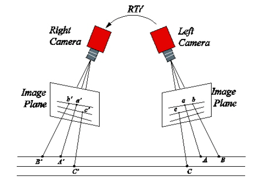
As the stereo measurement system can be treated as a special one of the multi-camera system, in our approach, we assume two cameras located in two different positions with non-overlapping view field.
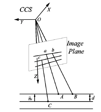
The structure of the measurement system is illustrated in Fig. 1.
The planar target used in our calibration method is required to be at least three parallel lines with equal space. The planar target should be located in the view field of each camera. When the target is formed into a rectangle, it is easy to satisfy this requirement. The images by each camera can be captured simultaneously.
The main steps of our calibration method are listed as follows:
1) The intrinsic parameters of each camera can be calculated by Zhang’s calibration method [8, 9]. The relative position between each two camera is unchangeable while the cameras are fixed in the proper position due to the requirement of the measurement. 2) The planar target with three equally space parallel lines is used to finish the calibration. Put the target in the view field of the two cameras simultaneously (as illustrated in Fig. 1). 3) Capture the image of the target from each camera separately, and then obtain the normal vector of the target plane in each camera coordinate system. So the rotation matrix of the two camera coordinate systems can be derived from the different expressions of the same vector, i.e. the normal vector of the target plane. 4) As the distance between each pair of adjacent parallel lines is known exactly, we can get some information about the translation matrix. When the target is moved into several different positions, enough consistency can be confirmed to calculate the translation matrix.
A set of parallels in 3D space projects on the image plane of perspective geometry and the intersection is called the vanishing point. The vanishing point depends only on the direction of the line rather than on its position. The vanishing point can be obtained by intersecting the image plane with a ray parallel to the line and passing through the origin of the camera coordinate system. By definition and using the principle of perspective geometry, we have the following property when the direction vector of the line is defined as

where
In [10], a new approach of calculating the vanishing line from three coplanar equally spaced parallel lines is proposed. When the homogeneous coordinates of the three parallel lines on the image plane are defined as

Moreover, we can obtain the relationship between the vanishing line and the normal vector of its corresponding plane:

where
2.2. Obtaining the Rotation Matrix
From the knowledge above, the normal vector of the target in the coordinate system of each camera can be derived from Eq. (3). Now the rotation matrix of the two coordinate systems can be obtained from the corresponding normal vectors using the method mentioned in [11, 12].
2.3. The Confirmation of the Translation Matrix
The normal vector of the target plane is known as and the direction vector of the parallel lines is , which is derived in Section 2.1. Furthermore, the perpendicular vector of the parallel lines on the target plane can be confirmed from the cross of the two vectors:

As illustrated in Fig. 2, three random points locating in two parallel lines are point
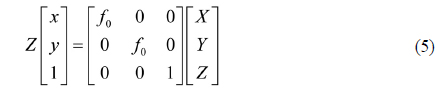
So the relationship between the image coordinate system and the camera coordinate system is:

where
Obviously, the direction vector from point

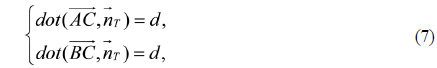
The projection of the vectors and onto the vector , which is the vertical vector of the parallel lines, is the distance

Combined Eq. (5) with Eq. (6) and Eq. (7), the coordinates of the points
Point

When the target is moved into more than two different positions, more equations like Eq. (8) can be obtained, from which we can derive the translation matrix simply.
III. SIMULATIONS AND DISCUSSIONS
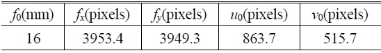
Simulations will be conducted to evaluate the impacts of some vital factors. The assumed multi-camera measurement system consists of two identical cameras, and the intrinsic parameters of each camera, which are listed in Table 1, are also identical.
[TABLE 1.] The intrinsic parameters of the camera

The intrinsic parameters of the camera
where
3.1. The Number of Target Positions
In the proposed method, one camera can capture one image of the target when the target is located in one position. And the normal vector of the target plane can be confirmed based on the property of the vanishing line. Theoretically, the rotation matrix can be determined by two vector pairs. But as the noise is inevitable, the normal will involve additive error. If more vector pairs can be used to confirm the rotation matrix, the additive error will be diminished. For the translation matrix, the number of target positions is the main factor, which can be obtained from the confirmation of the translation matrix. Therefore, the number of target positions is the only factor related to the translation matrix in this paper.
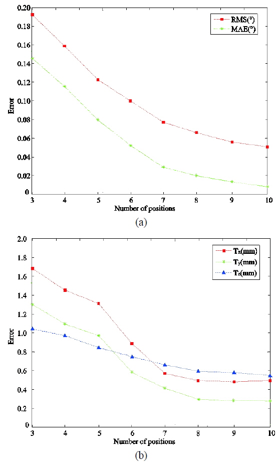
For the purpose of verifying the affection of the number of target positions, we conducted a simulation. In the simulation, the distance of each two adjacent lines is 20 mm, and the Gaussian noise with mean 0 and standard deviations of 0.5 pixels is added to the captured images. The number of target positions is varied from 3 to 10. In order to make the illustration clear, we transform the rotation matrix to the rotation vector and then calculate the angle between the ideal vector and the obtained one. The Root-Mean-Square (
It is obvious that the
3.2. The Distance between Two Adjacent Parallel Lines
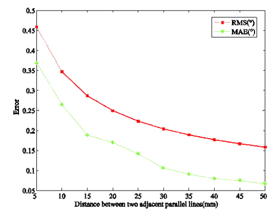
As it has been known, the normal vector of the target plane is determined by the parallel lines on the target. Nevertheless, when the distance between two adjacent parallel lines is large, the representation of the feature of vanishing is notable. In this case, the effect of the additive noise will be decreased. A simulation will be conducted to verify the conclusion. Similarly, the Gaussian noise with mean 0 and standard deviation of 0.5 pixels is added to the idealized ones to generate the perturbed images. The number of target positions in the simulation is 5. The distance between adjacent parallel lines varies from 5 mm to 50 mm with the interval of 5 mm. The criterion of the simulation is the same as mentioned in Section 3.1, the angle between the idealized rotation vector and the obtained one is used to measure the error involved in the determination of the rotation matrix. The
As illustrated in Fig. 4, the angle decreases as the distance between the two adjacent parallel lines increases. So it is appropriate to increase the distance if it is possible. Meanwhile, the distortion of the lens cannot be neglected, if possible, the parallel lines should form an image in the center of the image plane, while the increasing of the space may make it more difficult.
3.3. The Number of Points Used to Determine the Parallel Line
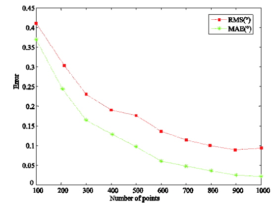
Obviously, the normal vector is one of the vital factors affecting the rotation matrix directly, while the normal vector is determined by the extraction of the parallel lines. In the proposed method, the extraction of the center of the line is based on C.Steger’s method mentioned in [13], which has the capacity of reaching sub-pixel accuracy. Then the function of the line can be determined by the fitting of the separate points. So the number of image points is another important factor affecting the calibration result. For this purpose, the related simulation has been conducted to evaluate the situation. In this simulation, the number of points used to fit each parallel line varies from 100 to 1000 points with the interval of 100 points. The distance between each pair of adjacent parallel lines is 20 mm, while the number of target positions is 5. The criterion evaluating the calibration results is the same as the description mentioned in Section 3.1, and the angle between the ideal rotation vector and the obtained one is the target. The related result is illustrated in Fig. 5.
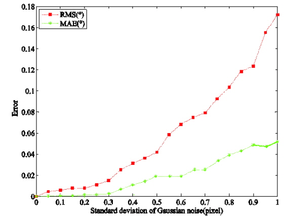
For the purpose of evaluating the practicability of the proposed method, the simulation will be conducted. Gaussian noise with different standard deviations is added to the ideal image to generate a perturbed one. The distance between the two adjacent parallel lines is 20 mm, while the number of target positions is 5. The rotation matrix is still evaluated by the RMS error of the angle between the ideal rotation vector and the obtained one. The translation matrix is evaluated by the absolute bias of each element. The calibration results are plotted in Fig. 6.
IV. THE REAL EXPERIMENT AND DISCUSSIONS
In the real experiment, the multi-camera measurement system consists of two cameras, which are
[TABLE 2.] The intrinsic parameters of the two cameras

The intrinsic parameters of the two cameras
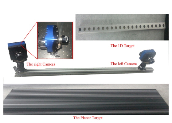
The target used in our experiment is a planar target with a series of parallel lines on it (Fig. 7), but actually, only three equally space parallel lines are used to determine the vanishing line, and further, the normal vector of the target plane.
Then the rotation matrix can be confirmed, while the translation matrix is determined by the steps described in section 2. According to the proposed method, the rotation matrix we obtained is , while the translation matrix is .
4.1. The Experiment for Repeatability
In order to verify the repeatability of the proposed method, we calibrate the multi-camera measurement system 8 times. In each time, the same experiment condition is requested. The standard deviation of the rotation vector and the translation vector are calculated, and the result is listed in Table 3.
[TABLE 3.] Experimental result of the repeatability

Experimental result of the repeatability
4.2. The Experiment for Determining the Accuracy
For the purpose of evaluating the accuracy of the proposed method, the method mentioned in Ref. [7] is used. Similarly, a 1D target with several feature points at each side is utilized (Fig. 7). The feature points on the left side are captured by the left camera while the feature points on the right side are captured by the right camera. As the constraint of the length, the coordinates of the feature points in each camera coordinate system can be determined. Then the feature points can be transformed to the right camera coordinate system according to the calibration result. The distance between the feature point captured by the left camera and the feature point captured by the right camera can be derived, while it is known exactly beforehand. The results are listed in Table 4.
[TABLE 4.] The accuracy test for the calibration result
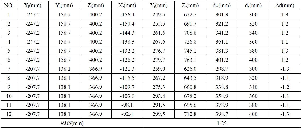
The accuracy test for the calibration result
[
In this paper, a new calibration method for the external parameters of the multi-camera measurement system is proposed. Using a target with three equally spaced parallel lines, the normal vector of the target plane can be confirmed. By moving the target into at least three different positions, the rotation matrix can be determined. As the distance between two adjacent parallel lines is known exactly, the translation matrix can also be obtained. Then all the external parameters are confirmed. The simulations and real experiments show that the proposed method is accurate and with good robustness. The calibration results can reach about 1.25 mm with the range of 0.5 m.
Moreover, as the feature of parallel lines exists widely, the proposed calibration method can also be used for auto-calibration. For instant, the natural feature of parallel lines, such as the edges of the windows or the building, can be utilized to finish the calibration, especially when the target is not proper or for a measurement system with a wide field of view.