Since white LEDs (light-emitting diodes) were invented in the1990’s, they have been extensively researched [1, 2]. Compared with the previous lighting devices, the white LED is more advantageous in terms of high brightness, lower power consumption, smaller size, longer lifetime, and environmental protection [3-5]. Because of these advantages, the white LED is considered as a strong candidate for the future lighting technology and will replace most of the conventional light sources in offices and homes [6-8]. Generally speaking, the LED lamps are not only used as a lighting device, but also to be used as a communication device [9]. The dual function of the LED lamps has aroused a lot of research interests in recent years. The lamp arrangement is one of the most critical issues in indoor VLC systems. It is known that a single LED lamp can’t provide sufficient illumination, so we tend to install several LED lamps on the ceiling to illuminate the room as evenly as possible. A lot of research has been done in the field [10-12]. And the research has shown that different LED lamp arrangements will have different illumination and communication quality, that is, both the lighting effects and the communication quality are closely related to the arrangement of the LED lamps [10, 13, 14]. Actually, in the same room, with the same number of the lamps, there is always an optimal arrangement, which can make full use of the LED lamps and gain the best uniformity. For the sake of simplicity, the word ‘lamp’ refers to ‘LED lamp’ in the rest of the paper.

The lamps can be, in principle, arbitrarily distributed, however, it is convenient to distribute regularly on the ceiling, for the purpose of uniform illumination. Most attention has been paid to the arrangement of 2 × 2. In the literature [4], for example, Toshihiko Komine et al. proposed a room model 5 × 5 × 3 m³, in which the size of the ceiling is 5.0 m × 5.0 m. This room model is called the square room model, since the plane where the lamps locate is square. Similarly, if the ceiling of a room is a rectangle, we called it a rectangular room model. In the proposed square room model, a method of determining the location of the lamps is to divide the ceiling plane into 2 × 2 parts and put one lamp in the center of each part. This method of determining the location of the lamps is easy, but not accurate or optimal. What we pursue is a method that can help to find the optimal arrangement accurately for any room model, such as the square room model, rectangular room model and so on. What’s more, when determining the locations of the LED lamps, the effect of reflection is always neglected, which make the results not so accurate for a real scenario. Actually, in a real scenario, the reflection is always there. According to literature [4], the ratio of the first order of reflection is 4.84 percent, which will exert influence on the arrangement of the lamps. So, in order to gain the optimal arrangement accurately, the first order reflection is taken into consideration when determining the location of the lamps. And in the calculation, the Multi-Input Multi-Output (MIMO) system model is applied to reduce the amount of calculations.

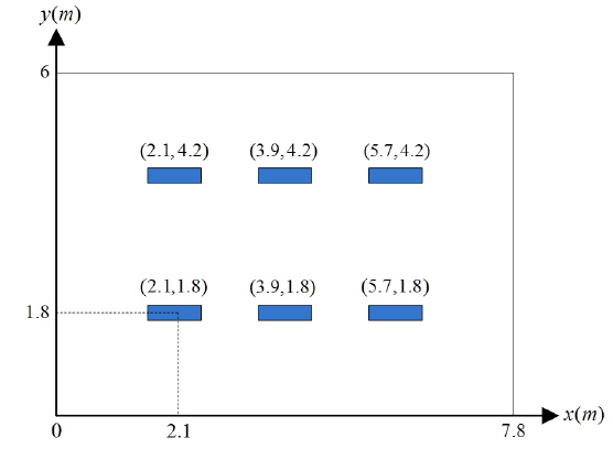
In addition, the previous research has been mainly based on the square room model, as far as we know, no study of the rectangular room model is available. However, in the real environment, the rectangular room model is more common, so we choose a rectangular office room scenario for our study, in which 2 × 3 lamps distribute on the ceiling symmetrically. The real scenario is illustrated schematically in Fig. 1. Since the most important and common target illumination function in daily life is still uniform distribution around the room. Hence, in this paper, we focus on the uniform illumination distribution by the 2 × 3 lamps, with other environmental parameters unchanged.

To get the best uniformity, we propose a method to calculate the optimal location of the lamps and to gain the optimal arrangement, in which the first order reflection is taken into consideration. In literature [14], the received optical power is used to analyze the optimal arrangement. Since the distribution of illumination has the same shape as that of the received optical power when the FOV is 90 degrees, so the optimal arrangement would be the same no matter whether illumination or received optical power is used to analyze the lamp arrangement. In this paper, we focus on analyzing the optimal arrangement from illumination. Under the optimal arrangement, a better illumination distribution is achieved, which proves the validity of the method. Meanwhile, when the lamps work as a communication device, the optical signals of the lamps travel via different paths and arrive at the receivers at different intervals in time. The optical path difference between the multiple sources triggers inter-signal-interference (ISI), which will significantly degrade the performance of the indoor VLC system [1, 9]. To judge the influence of the optimal arrangement on the communication quality, the root mean square (RMS) delay spread is studied, which is a better measurement for the spread of multipath and can predict ISI accurately [1, 15]. Simulation results indicate that the fluctuation of the RMS can be mitigated by the optimal arrangement, comparing with the original lamp arrangement.

The rest of this paper is organized as follows: in Section Two, the principle parameters of LED, the real office room scenario and illumination distribution are presented. In Section Three, the method to gain the optimal arrangement is introduced and the optimal arrangement of the office room is presented. Section Four shows the simulation results under the optimal arrangement, including the illumination distribution and the RMS delay spread distribution. Finally, Section Five presents the conclusion.

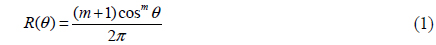
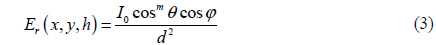
LED has two basic properties, a luminous intensity and a transmitted optical power. The relationship between photometric and radiometric quantities is explained in [16, 17]. In this paper, the Lambertian radiation pattern is applied to model the LED radiant irradiance [14].

Where, θ is the angle of irradiance from the LED lamp, m is the order of Lambertian emission and is defined by the semi-angle at half illuminance of an LED lamp θ_1/2 as = -ln2 / ln(cosθ_1/2), especially, when θ_1/2=60°, the corresponding value is 1.

The luminous intensity in angle θ is given by [4]

A horizontal illumination E_r at a point (x, y, h) is given by

Where, I₀ is the center luminous intensity of an LED, φ is the angle of incidence, and d is the distance between an LED transmitter and a receiver’s surface. The illumination expresses the brightness of an illuminated surface.

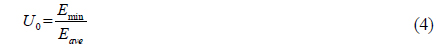
The consideration for illumination of LED lighting is required. Generally, illuminance of lights is standardized by the International Organization for Standardization (ISO). According to this set of standards, illuminance of 300 to 1500 lx is required for office work [4].

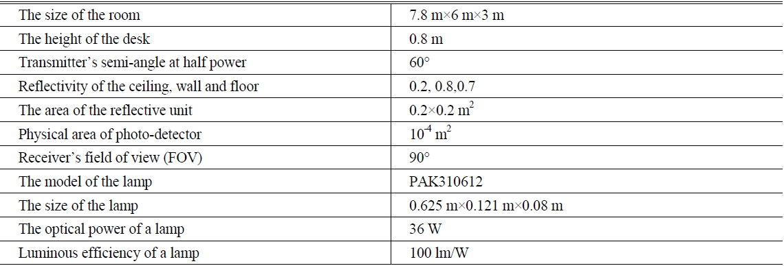
In this subsection, the room scenario we choose and the illumination distribution under the original arrangement is introduced. The size of the office room is 7.8×6×3 m³. The lamps are installed at the height of 3.0 m from the floor. The height of the desk is 0.8 m, and the receiver is put on the desk. The number of the lamps is six. Each lamp has a total luminous flux of 3600 lm, and the transmitted optical power 36 W. These represent the measured and calculated values of the commercial product PAK310612 PAK-A02-118-DZ. It has a size of 0.625 m × 0.121 m × 0.08 m. The ceiling, wall, and floor have reflective index values of 0.2, 0.8, and 0.7, respectively. The conditions are summarized in Table 1.

Here, we define the x-y plane as a plane parallel to a floor face, and the z-axis as a height direction. As shown in Fig. 1, the central position of the lamps are (2.1, 1.8, 3), (2.1, 4.2, 3), (3.9, 1.8, 3), (3.9, 4.2, 3), (5.7, 1.8, 3) and (5.7, 4.2, 3). This arrangement is called the original arrangement. Note that in the simulation, to closely approximate the real scenario, the size of the lamp is considered.

In the original arrangement, the six lamps mainly concentrate in the central areas of the room, which will result in larger illumination in the central areas and smaller illumination in the areas close to the walls. The great fluctuation will limit the system’s ability to provide equal lighting effects for the users in any place in the office. Here, uniformity U₀ is used to evaluate the fluctuation of the light distribution, which is defined as

Where, E_min is the minimum illumination, E_ave is the average illumination on the receiving plane, which refers to the 0.8 m plane of the office room in this paper. The higher the U₀ is, the more uniformly the illumination is distributed in the room. The maximum of U₀ is 1, which is only theoretically possible, in practice impossible, but we can try to get close to it. When U₀ is closer to 1, the uniformity of the illumination distribution is considered to reach a better state. Generally, U₀ should be over 0.7 according to lighting engineer [1].

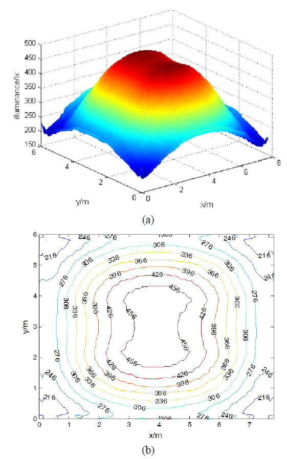
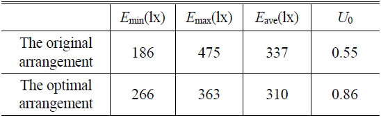
The distribution of horizontal illumination under the original arrangement is shown in Fig. 2, where the minimum and the maximum are 186 lx and 475 lx, respectively. And the U₀ is only 0.55, which means the value of illumination varies substantially in the room, i.e., the lighting’s effect is associated closely with user’s location. The users in the corner of the office will obtain less than 60.8 percent (289 lx) of the illumination in the center of the room. That is, only the central regions of the room can meet the requirement of 300-1500 lx, according to ISO. Note that in the simulation, the reflections of the wall, the ceiling and the floor are considered.

The poor illumination distribution in Fig. 2 is caused by the unreasonable arrangement of the lamps: the six lamps are mainly concentrated in a small region of the center. The distance between the lamp source and the receivers in the central regions is much shorter than the receivers in the corners. According to equation (3), the intensity in the central areas is definitely much higher than that in other places, which, finally, lead to the un-uniformity of the illumination. So we try to rearrange the location of the lamps.

In this part, we will introduce the theory of optimal lamp arrangement taking the first order reflection into consideration. Note that in this paper, all the lamps point vertically to the plane where the receiver is located. And the lamp is assumed to be a point source when calculating the optimal lamp arrangement.

In the receiving plane, the total illumination E_r at a point (x, y, h) due to the multiple lamps is the superposition of the illumination of the lamps with potentially different illumination distribution depending on their positions [1]. E_r is expressed as

Here, E_i refers to the horizontal illumination of each lamp. Generally, E_i should contain the illumination of the directed path and all of the reflected paths. Since the ratio of all the reflection is 4.84 percent, in which the first order of reflection accounts for 3.57 percent and the reflection effects weaken with the increasing of the orders of reflections [1, 4]. Thus, we only consider the first order of reflection when calculating the optimal arrangement, which is enough to accurately simulate the real scenario. Assume that the number of the lighting sources, the receivers and the reflective units are t, r and n, respectively. According to the MIMO system model, the illumination on the receiving plane can be expressed as [18]

Where, P is the optical power of a lamp, η is the luminous efficiency of a lamp. D_t×r, F_t×n, and M_n×r, are all matrixes. D_t×r represents the response from the source to the receivers directly, and the product of the matrices F_t×n and M_n×r represents the response through the first order of reflection. F_t×n is the transfer function between the lighting source and the reflective units, and M_n×r is the transfer function between reflective units and receivers. D_t×r can be expressed as

Here, d_ik correspond to the illumination from lamp i to receiver k, which can be easily calculated by equation (3).

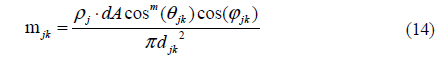
To calculate the illumination from reflection, we make the following assumptions: to model the reflection from a differential reflecting unit with area dA and reflectivity ρ , and first consider the small unit as a receiver with area dA and calculate the luminous intensity it receives, and second model the different small reflector as source and an ideal Lambertian radiation intensity pattern, as given by equation (1). The other parameters are listed in Table 1.

Since the reflective surfaces do not offer perfect reflection, and illumination is inversely proportional to the distance that light travels, a finite unit number of reflective units is considered in calculating the illumination from the reflective planes. And in our discussion, we assume the internal surface is made up of n neighboring units of equal area. Generally speaking, the smaller the area of the reflecting unit, the more accurate the simulation result is. However, the numerous units would increase the run time. Sometimes it can be several days or years. Reducing the number of the units would shorten the run time at the expense of reduced accuracy. So a modest number of reflective units would be better. For a room with a size of L×W×H, the total number of the reflective units is then given by [19].

Where,

Here, d is the distance between centers of neighboring units, which is taken to be the same for all surfaces. In this paper, the reflection planes are divided into small unit, with d is 0.2 m. In addition, since the receiver is put on the desk, the reflective units that are lower than the desktop will not contribute to the illumination. Thus, we only consider the reflective units that higher than the desktop, which can help to shorten the simulation time and meanwhile, maintain the accuracy of the calculation. Thus, equation (9) can be rewritten as

Here, h is the height of the receiving plane. And in this paper, h is 0.8 m. The transfer function F_t×n is given by

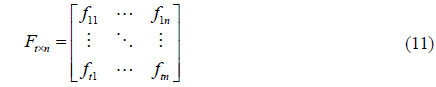
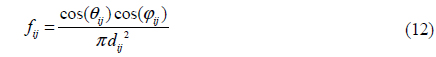
Since reflective units 1 through n receive the illumination directly, the transfer function f_i×j between a lighting source i and unit j can be obtained from equation (3), and is given by

Where, cos(θ_ij) is equal to dot product of two unit vectors. The first is perpendicular to the source i, and the second originates from source i and extends toward reflective unit j. The angle φ_ij is the angle between a vector perpendicular to reflective unit j and a vector that lays on the straight line that connects source i and reflective unit j. d_ij is the distance between the source i and the reflective unit j.

And the transfer function M_n×r can be expressed as:

Here, m_jk is given by

Where, ρ_j is the reflection factor of the reflective unit, dA is the area of the reflective unit j, θ_jk is the angle between the normal vector of the jth reflective unit and direction vector from the jth reflective unit to the kth receiver, φ_jk is the angle between the normal vector of the kth receiver and direction vector from the kth receiver to the jth reflective unit. d_jk is the distance between the jth reflective unit and the kth receiver. Once the matrices D_t×r, F_t×n, and M_n×r are determined, the illumination on the receiving plane can be gained by equation (6).

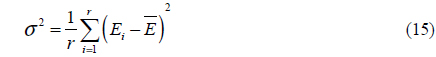
Different arrangements will lead to different illumination distributions. To evaluate whether the arrangement is good, here, we introduce the variance of the illumination intensity. When the value of the variance reaches the minimum, the illumination distribution will be the most uniform one. Then we regard the arrangement as optimal. The variance is defined as follows.

Here,

Where, r is the number of the receivers on the receiving plane, E_i is the illumination the ith receiver receives, is the average illumination. Both of them can be gained from the matrix E_t×r easily. The smaller the variance is, the smaller the fluctuation of the illumination distribution, which means better uniformity.

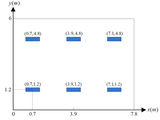
A computer program is written to implement the algorithm described above. Since the location of the lamp is symmetric with respect to the center of the ceiling. To keep the symmetry, we fix two of the lamps on the ceiling with their abscissa both at 3.9 m, as shown in Fig. 3. So assuming the location of the first lamp is (x₀, y₀, 3), then the coordinates of other lamps can be expressed as (x₀, 6-y₀, 3), (3.9, y₀, 3), (3.9, 6-y₀, 3), (7.8-x₀, y₀, 3), and (7.8-x₀, 6-y₀, 3), respectively. With the value of the x₀ and y₀ changing, the arrangement will be different. Under different lamp arrangements, there will be a different illumination matrix E_t×r, and variance. Note that, in the simulation, t is 6, and we are assuming that there are 26×20 receivers on the receiving plane, that is, r is 520. The ranges of the x₀ and y₀ are both 0 to 2. By computer simulation, we find that when x₀ is 0.7 m, and y₀ is 1.2 m, the variance reaches the minimum. Thus, when x₀ is 0.7 m, and y₀ is 1.2 m, the optimal lamp arrangement is gained. The optimal arrangement is shown in Fig. 3. We can see that the lamps are no longer concentrated in a small range of the center, but scatter near the wall, which can help to achieve a better uniformity. Note that the optimal arrangement is not affected by the value of lamp power. Once the dimensions of the room, the reflection units and the lamps are determined, the optimal lamp arrangement is determined, regardless of the power of the lamps.

In this subsection, the distribution of horizontal illumination under the optimal lamp arrangement gained in Section Three will be discussed. To ensure that the results are consistent with the practical situation, the reflection of the walls, the ceiling and the floor are considered. The reflective factor is listed in Table 1. To compare with the illumination distribution under the original arrangement, the environment of the room, the total number of lamps and power of each lamp remains the same.

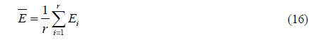
Figure 4 shows the illumination distribution under the optimal arrangement. The illumination ranges from 266 lx to 363 lx. It can be seen that the maximum illumination doesn’t occur in the center of the room, but occurs in the areas under each lamp. It is because the lamps are not concentrated in a smaller range of the room any more, but are closer to the walls. With the distance between the lamps and the receivers reduced, the receivers close to the walls can receive more light, which helps to mitigate the fluctuation of the illumination. Table 2 shows the comparison in illumination distribution between the original arrangement and the optimal arrangement, it can be seen that compared with the original arrangement, the uniformity U₀ increase from 0.53 to 0.86, which means the illumination distribution is more uniform and the lighting effects in different places are not so associated with the user’s location. Note that when the power of lamp changes, the uniformity would not change, as long as the arrangement of lamps is as determined. For example, when the power of lamp increases to 72 W, the average illumination increases to 619 lx, while the uniformity is still 0.86. In this paper, we mainly focus on the performance of the uniformity. So though the average illumination decreases from 337 lx to 310 lx comparing with the original arrangement, the arrangement is optimal, since the uniformity of the illumination is improved greatly.

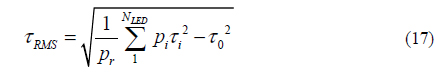
Uniformly-distributed illumination is very important when the lamps work as lighting devices. The RMS delay spread is also desired when considering the communication function. In the indoor VLC system, the signal transmitting path is directly relevant to the transmitters, that is, the locations of the lamps. When the lamps transmit the same signals synchronously, the receiver on the desk receives the signals from different lamps. Since the transmitting path is different, the time at which the signals arrive is different. The path delay of the same signal will lead to ISI, which is sure to deteriorate the quality of communication. A useful measure of the severe ISI induced by a multipath channel is the root mean RMS delay spread τ_RMS. The RMS delay spread is defined as [15]

Where, p_r refers to the total received power from all the lamps, p_i is the received power of the ith path, τ_i is the time delay of one path, τ₀ is the mean delay of all the paths. It is given as

Where, p_i = p₀H(0), and , N_LED is the number of the lamps, the corresponding value is six in this paper. RMS delay spread represents an effective delay of the channel impulse response, and it is a remarkably accurate predictor of ISI. It varies in the level of ns. The smaller the value of τ_RMS is, the better the quality of communication.

Figure 5 shows the distribution of RMS delay spread under the original arrangement, where the RMS delay spread of visible light varies between 0.96 ns and 3.64 ns. The worst RMS delay spread occurs at the edge of the room, and the least RMS delay spread occurs in the center of the room. It means that when a user moves from a place in the center to another in the corners of the room, the quality of the communication quality will decline sharply. That is unfair for the user not in the central places of the office. 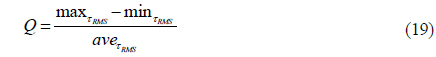To measure the fluctuation of τ_RMS in the receiving plane, a variable Q is introduced, which is defined as

Where, max_τRMS and min_τRMS are the maximum and the minimum of the RMS delay spread, respectively, and ave_τRMS represents the average of the RMS delay spread on the plane where the receiver is located. The smaller the Q is, the smaller the fluctuation of the RMS delay spread on the receiving plane.

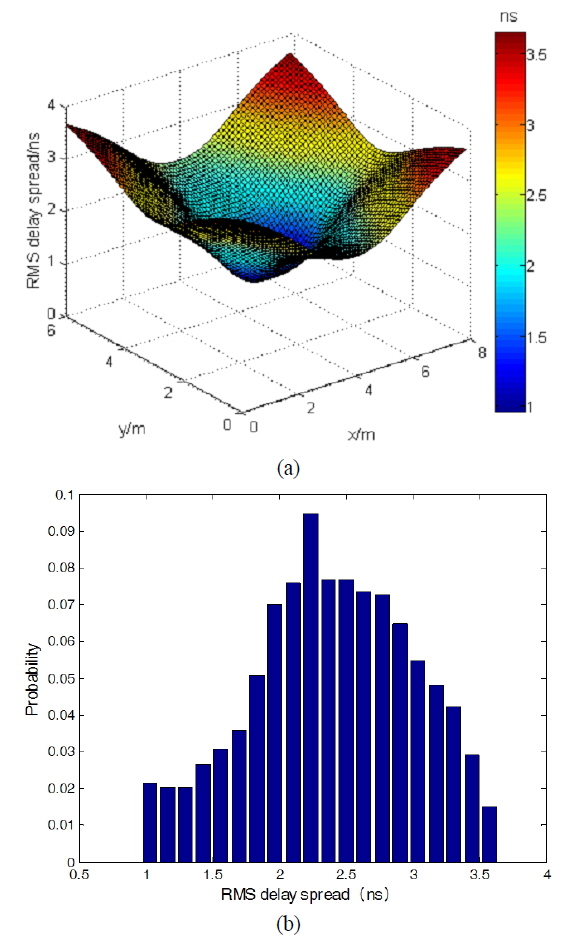
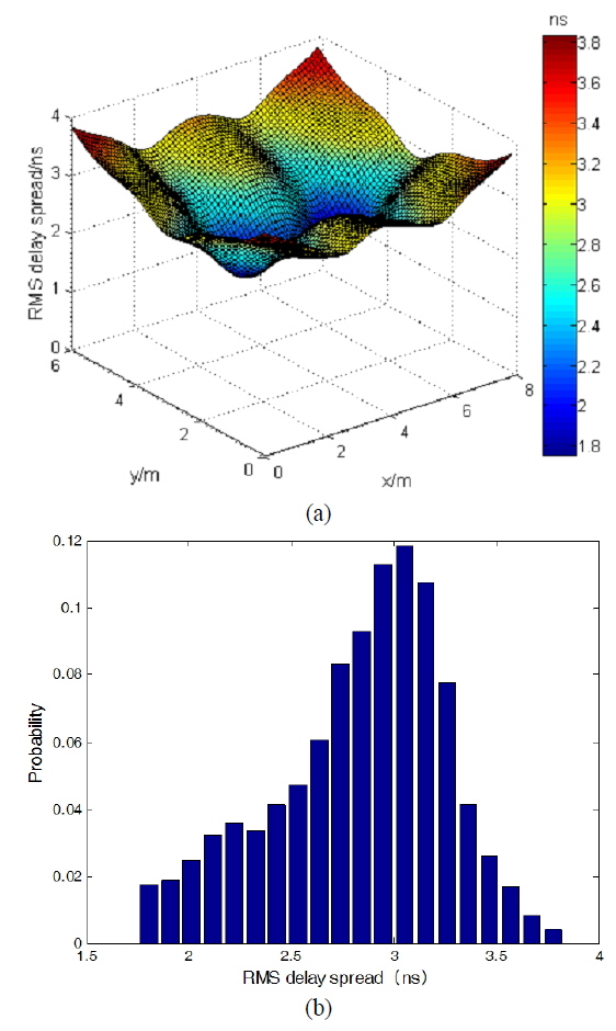
In Fig. 5, the maximum RMS delay spread is about 2.7 times higher than the minimum. And the value of the Q is only 0.4, which means a great fluctuation of the RMS delay spread. The fluctuation will limit the system’s ability to provide equal communication quality to multi-users in different places. The poor performance of RMS results from the unreasonable lamp arrangement. Generally, a reasonable arrangement can mitigate the fluctuation. Figure 6 shows the RMS delay spread under the optimal arrangement. We can see the fluctuation is not so obvious and the value of the Q increased from 0.4 to 0.62, increased by 55 percent. As shown in Fig. 6 (b), the probability of the smaller RMS delay spread is much higher than that in Fig. 5 (b).

Though the fluctuation can be mitigated under the optimal lamp arrangement, we must note that there is still a big difference between the maximum and the minimum and the average RMS delay spread increases from 2.39 ns to 2.83 ns, which will not be beneficial to the improvement of the communication quality. It is because in the real scenario, the lamp is not a point light source, but has a certain size, as shown in Fig. 1, while when calculating the optimal locations, the lamps are considered as point light sources for the sake of simplicity. In addition, in this paper, our studies mainly focus on the fairness in providing equal lighting effects and communication quality for the users in any place of the room. So, the Q is more desired. What’s more, the increase of the average is smaller compared with the improvement of the Q. Based on these reasons, though the results are not so perfect, it is still a strong proof that method we proposed to calculate the optimal arrangement is reliable, since under the optimal arrangement, not only the fluctuation of the illumination but also the fluctuation of RMS delay spread is mitigated greatly.

In this paper, we have investigated and studied the LED lamp arrangement, and analyzed the illumination distribution by using a rectangular room model, in which there are 2×3 lamps distributed symmetrically in the ceiling plane. In the analysis, we applied the MIMO system model in our work and proposed a method to determine the location of the lamp taking the first order reflection into consideration, and finally, we gained the optimal arrangement. Under the optimal arrangement, the illumination and RMS delay spread distribution were analyzed. The simulation results show that compared with the original arrangement, the uniformity of the illumination can be improved from 0.55 to 0.86, which ensures almost equal lighting effects for all users at different locations in the room. Meanwhile, the dramatic change of RMS delay spread that incurred by the unreasonable lamp arrangement is mitigated by the optimal lamp arrangement from 0.4 to 0.62.