In 1964, the first geostationary Earth orbit (GEO) satellite, Syncom-3, was launched by a Delta D rocket. GEO satellites can be used for communication and broadcast services for commercial and public use. GEO is defined as a restricted area 42,164 km from the center of the Earth and on the celestial equatorial plane, so the number of possible GEO satellites is limited. After a satellite is retired, the Inter-Agency Debris Committee (IADC) recommends re-orbiting it outside of the protected region. For GEO, the protected region, Region B, was defined as the GEO altitude plus or minus 200 km and the equatorial latitude plus or minus 15° of arc (IADC 2014). Further, satellite operators usually maneuver GEO satellites to a fixed station-keeping area.
Collision avoidance is an important issue for the operation of a GEO satellite. Space debris such as rocket bodies and materials and obsolete or uncontrolled satellites can be hazardous to active satellites. The lifetime of space debris at high altitudes exceeds 1,000 years. However, objects at high altitude drift to stable points because of geopotential perturbation (Soop 1994). As the position of active satellites is maintained by station-keeping maneuvers, their orbital revolutions differ from those of space debris or drifting satellites. This increases the possibility of collision between active satellites and other high-altitude objects. For effective protection of active GEO satellites, the orbital revolution of high-altitude objects should be monitored by survey observation at appropriate intervals (Jo et al. 2011; Rahoma et al. 2014).
Schildknecht et al. (1997) analyzed the possibility of optical observation of space debris using the Zimmerwald Laser and Astrometry Telescope. Their experiments focused on the effectiveness of an observation strategy to find space debris in the GEO protected region. Africano et al. (2000) proposed a GEO object search strategy to overcome narrow field of view (FOV) and brightness limitations. Subsequently, a GEO survey observation was made using the 1-m optical telescope at Tenerife, and highly eccentric orbit survey results were also presented (Schildknecht et al. 2001a, 2004). A survey network was also simulated to survey the entire GEO region and maintain the catalog (Flohrer et al. 2005). Flohrer et al. (2008) proposed optical observation strategies for not only highly eccentric objects but also low Earth orbit and medium Earth orbit objects in the European Space Surveillance network. Catalog correlation is another concern in identifying observed objects from survey observation results. Früh et al. (2009) applied a new correlation method to typical GEO and Geostationary transfer orbit (GTO) survey observation from the European Space Agency Space Debris Telescope (ESASDT) at Tenerife. Olmedo et al. (2009) presented a correlation technique for optical and hybrid measurements to maintain a space surveillance system catalog. Further, a multi-telescope site for the survey network was designed and developed, and an observation strategy using it was analyzed (Olmedo et al. 2011).
Maintenance of the satellite catalog also requires an orbit determination procedure. Survey observation focus on the detection of correlated and uncorrelated objects, their identification, and analysis of their orbital information (Choi et al. 2009b). As the number of survey observation measurements is smaller than that of normal target observation measurements, the orbit determination accuracy is important for effective catalog maintenance. Kawase (2000) investigated the theoretical error of GEO satellite orbit determination using angle-only measurements for a single-day and multi-day observation. Musci et al. (2004) used sporadic-case measurement for initial orbit determination and improved it by follow-up observation measurements for a few days. They also examined the orbit determination error with follow-up observations at 30 and 120 days (Musci et al. 2005). Choi et al. (2009a) proposed a simple survey strategy considering the accuracy of an initial orbit determination for GEO catalog objects that can be observed at a Daejeon station. Milani et al. (2011) presented an improved initial orbit determination result by using an admissible region and a least square method with survey observation data obtained at the 1-m ESASDT. On the other hand, Tombasco & Axelrad (2011) and Choi et al. (2015) analyzed the orbit determination accuracy using angle-only measurements for various observation scenarios. The detailed orbit determination analysis results are useful for development of an effective survey strategy.
The brightness of space objects is very important for optical satellite tracking. Space debris, which is smaller than typical satellites, is relatively faint, and the brightness varies irregularly because the attitude is not controlled. Schildknecht et al. (2001b) revealed that the brightnesses of cataloged space objects were distributed around magnitude 12.5. Choi et al. (2011) also analyzed the brightness of 70 GEO satellites that can be observed in Daejeon and found that their average brightness is magnitude 10.75 ± 0.63. Further, Seo et al. (2013) mounted an observational campaign to confirm the brightness of the Communication, Ocean, and Meteorological Satellite (COMS) and its variation. Although the COMS is relatively small compared with other domestic communication satellites, its average brightness is magnitude 14.
We analyzed observation strategies to protect active geosynchronous orbit (GSO) satellites. GTO objects were ignored. The status of the GSO region was analyzed for the development of a survey observation strategy. The two-line element sets (TLEs) provided by the Joint Space Operation Center (JSpOC) were used to describe the orbital characteristics of GSO satellites. Active and inactive satellite were considered separately to meet the objective of the survey observation. Next, the GSO survey strategy was evaluated using four observation scenarios for active and inactive GSO satellites. We defined the observation systems in terms of the FOV and observation interval. Observation coordinates were simulated under the optical tracking conditions in Daejeon. The System Tool Kit (STK) was used to generate an ephemeris of the GSO satellites for a one-day test. We attempted a survey simulation using the observation scenarios and the ephemeris to determine the detection rate. The simulated detection efficiency was analyzed, and an optimal survey scenario and system specification were selected. An orbit determination strategy using the optimal survey conditions for GSO catalog maintenance was evaluated. A tasking observation strategy to maintain the orbital information of the cataloged satellites was also considered. For the survey observation, the orbit determination could be processed using sparse-case optical measurements. Finally, we suggest an survey observation strategy, including the system specifications, and the potential for maintaining the entire GSO catalog.
Analysis of the status of the GSO region is needed for development of an effective survey strategy. GSO is a spatially limited orbit because the revolution period is the same as the Earth’s rotation period. Most active GSO satellites are fixed near the space over their country of origin for broadcasting and communication. For active GSO satellites, station-keeping maneuvers and attitude control are performed by the owner or operators. In contrast, inactive satellites are affected by geopotential perturbation without any control, so they drift to stable points with time. A satellite maneuver can result in an unexpected situation, and we can detect space objects that pose a hazard to active satellites by analyzing the distribution and orbital trend of GSO objects (Lee et al. 2012).
The STK software from Analytic Graphics Inc. was used to analyze the status of the GSO protected region. GTO objects were also counted in this analysis. In the STK, high-altitude objects are classified as active, inactive, or decayed. Active objects included partially active, spare, and backup/standby cases. On April 10, 2015, the numbers of each type were 424, 518, and 12, respectively. The decay case was analyzed in the same way as the inactive case. Only 288 of the inactive objects had a circular orbit. The orbital characteristics of each case were generated using the STK and TLEs from JSpOC.
The orbital distributions of GSO objects were analyzed using TLE data from JSpOC. Fig. 1 shows the distribution of GSO objects in a plot of the semi-major axis versus the eccentricity. Active GSO objects have almost the same semimajor axis, but the eccentricity ranges from 0 to 0.005.
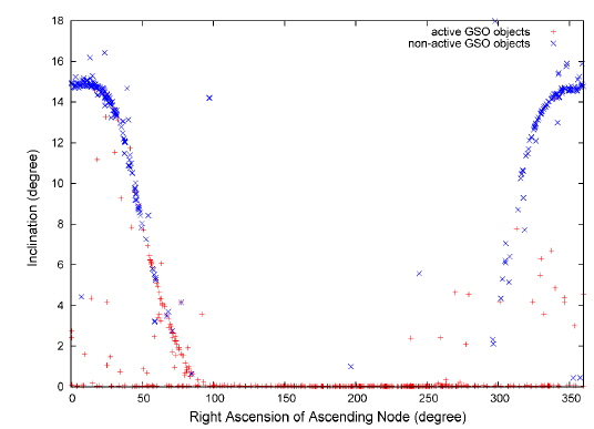
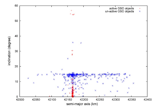
A plot of the semi-major axis versus the inclination (Fig. 2) shows that the inclinations of many inactive GSO objects reach 15°. The inclinations of active satellites are generally less than 15°, although some have inclinations as high as 60° depending on their mission. The right ascension of the ascending node (RAAN) and the inclination of GSO objects evolve under precessional motion. The inclination varied between 0° and 15° with a period of about 53 years (Schildknecht et al. 2001a).
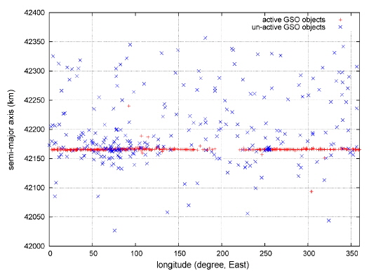
The longitudinal variation of the GSO objects was analyzed in terms of the semi-major axis. Fig. 3 shows that most of the GEO slots contain multiple satellites, but the region near a longitude of 201° is relatively empty. This region is over the Pacific Ocean. In contrast, inactive GSO objects have a wide range of longitudes and semi-major axes. In the GEO region, two stable points exist at longitudes of 75.1° and 254.7°. In addition, two unstable points exist at longitudes of 161° and 348°. GEO objects drift to the stable points. For example, objects west of longitude 161° are drifting toward the stable point at 75.1°. However, objects east of longitude 161° are drifting toward the stable point at 254.7°. Because of geopotential variation, the drift rate has a gradient depending on the longitudinal position (Soop 1994).
Fig. 4 shows the distribution of GSO objects on a plot of the inclination versus the RAAN. Most active GSO objects have various RAANs, but some active GSO objects and most inactive GSO objects have a RAAN between 300° and 100°. The typical RAANs of inactive GSO objects are centrally distributed near 0°.
3. SIMULATION OF OPTICAL SURVEY OBSERVATION
A Survey observation at a single optical tracking site was simulated to analyze the observation efficiency. The site was located in Daejeon, South Korea, and the epoch was April 10 (1 day). To simulate realistic observation environments, the STK was used with three limits on the optical tracking. The elevation limit was set to 10°, and the solar elevation limit was −3°. In addition, satellites that were observable within the penumbra of the Earth or in direct sunlight were chosen. The maximum observation time at the site was 10.7 hr under these conditions. Northern or southern sites generally have a smaller observation window for the GEO region than a site on the equator (Flohrer et al. 2005). For the Daejeon site, the observable longitudinal range is approximately 107° for GEO satellites. The numbers of observable active and inactive satellites are 152 out of 412 and 135 out of 288, respectively.
We assumed four optical tracking systems with two sizes of FOV and two observation intervals. In many cases, general astronomical telescope systems have been used for GEO satellite surveys considering the brightness and angular rate of motion of GSO objects. The FOV of the observation system was selected to be 1° or 2°, which is larger than that of a typical telescope but not larger than that of a dedicated system. Observation intervals of 2 sec and 5 sec were chosen to obtain an adequate signal-to-noise ratio (SNR). If the primary mirror of a telescope is more than 1 m in diameter, most GSO satellites can be observed. In this case, objects down to magnitude 18 can be imaged with a sufficient SNR on a clear night (Flohrer et al. 2005). Observation scenarios were simulated for these optical tracking systems. System 5s_1d denotes the optical system with a 1° × 1° FOV and 5 sec time interval.
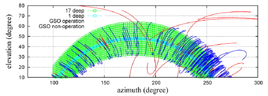
The simulated target coordinates were essentially along GEO. Further, the vertical range of the coordinates was increased as the elevation range (“deep”) increased. To cover the target coordinates, the telescope mount first moves vertically in the elevation direction and then covers the same pattern in the adjacent column of the elevation range. We can revisit the same area using this method. Fig. 5 shows the simulated coordinates and motion of GSO satellites in the sky. The simulated coordinates of the GEO and an FOV of 2° × 2° within 17 elevation intervals and 1 elevation interval are denoted by sky-blue and green open squares, respectively. The motions of active and inactive GSO satellites are indicated by red and blue dots, respectively. The observation conditions were applied to the motion of the satellites. The motions of some inactive GSO satellites show discontinuities caused by the Earth’s shadow. The simulated coordinates show good coverage of all the inactive GSO satellites’ motions for the region that is due south, but insufficient coverage of the eastern and western sides. Thus, only the vertical motions were considered to prevent distortion of the coordinates.
Table 1 shows the duration for one set of observations. The required time for one set of observations with a 1°×1° FOV and 5 sec interval is 16.25 min. In contrast, the telescope with a 2° × 2° FOV and 2 sec interval can make one set of observations in 3.03 min. At the end of one set of observations, the observation with the same coordinate set was repeated. The number of sets and the elevation range are inversely proportional, and the minimum number of required set is three for the initial orbit determination.
[Table 1.] Observation duration (minutes) for one cycle of various observation types.
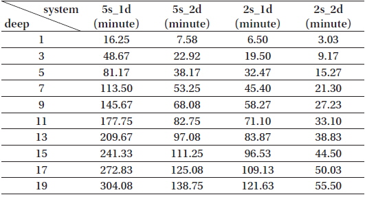
Observation duration (minutes) for one cycle of various observation types.
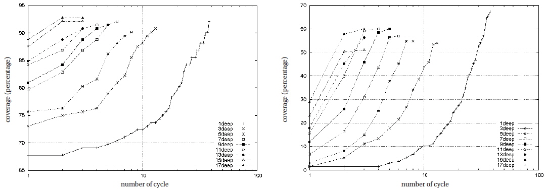
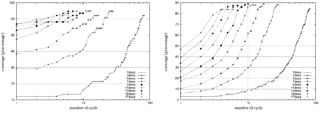
The detection rates of each observation scenario were calculated using the observation simulation program and the STK. Active and inactive satellites were considered separately to confirm the orbit determination strategy. The primary objectives of active satellite observation to maintain the orbital information are simulated. For inactive satellite observation, checking the probability of collision with active satellites and detecting unknown objects are important issues. Fig. 6 shows the detection rates of simulated observation with the 5s_1d system. The detection rates after only a few sets are very low because of the large inclination of inactive GSO satellites. For active GSO satellites, the maximum detection rate does not exceed 93%. This is attributed to the fact that some GSO satellites have inclinations greater than 15° to meet their mission objectives. The detection rate is proportional to the number of sets but decreases as the number of sets increases. The reason is that the motion of some of the GSO satellites extends beyond the simulated observation area. The detection rate is affected most strongly by the elevation range of the observation. Making more sets can increase the detection rate, as shown in the inactive GSO simulation for one elevation interval.
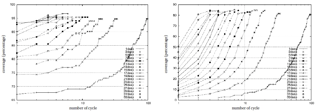
The detection rates of the 5s_2d system (Fig. 7) are generally higher than those of the 5s_1d system. The detection rates of inactive GSO satellites are approximately 20% greater, and the results for active GSO satellites show similar trends at 13, 15, and 17 elevation intervals. For inactive GSO satellites, the detection rates in a greater elevation range are lower than those in a smaller elevation range when the number of passes is greater. The active GSO satellite simulation at 13 elevation intervals shows the maximum detection rate at six sets. The total observation duration is 9.6 hr. However, the active GSO satellite simulation at 7 elevation intervals and 11 sets shows a maximum detection rate similar to the result for 13 elevation intervals. The total observation duration is 8.3 hr. The inactive GSO satellite simulation with 9 elevation intervals shows the maximum detection rate at 10 sets. The total observation duration is 10.7 hr, which is same as the total observable duration for this site.
To increase the detection rate in the survey observation, the optimal elevation range and number of sets should be determined. A wide FOV is naturally more efficient. The optimal observation strategy can reduce the observation time. The optimal size of the elevation range is proportional to the distribution of the inclinations of the observation targets. Further, the detection rate depends on the number of sets, but the elevation range is the dominant factor.
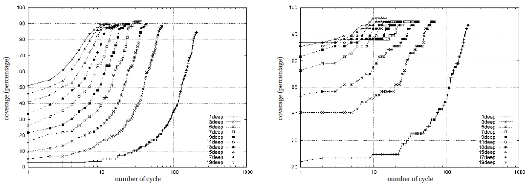
A survey observation strategy using a 2 sec interval was also tested to check the detection rates. Simulations of the 5s_nd systems show that the FOV and observation frequency are proportional to the detection rate. Fig. 8 shows the simulated detection rates for the 2s_1d observation system. In comparison with the 5s_1d system, although the detection rate is lower at the same number of sets, the maximum detection rates are higher. For the active GSO satellite simulation, an observation strategy with 19 elevation intervals shows the maximum detection rates, and the results with a wide elevation range are similar. In the inactive GSO satellite simulations, the elevation range is proportional to the detection rate. The initial detection rates for the observation strategy using the 2s_1d system are similar to the results of the 5s_2d system. The elevation ranges at 33 elevation intervals for the 2s_1d system and 17 elevation intervals for 5s_2d are 30.7° and 32.4°, respectively. Furthermore, the maximum detection rate of the 5s_2d system is higher than that of the 2s_1d system.
The final simulated observation system is the 2s_2d system, the detection rates for which are shown in Fig. 9. The active GSO satellite simulation with 10 elevation intervals shows the maximum detection rate for 10 passes. The total observation duration is 9.25 hr. Further, the detection rates are similar if the number of elevation intervals exceeds 13. For inactive GSO satellites, the elevation range is strongly proportional to the detection rate, as before. The detection rate is maximum for 7 elevation intervals and 28 sets, which requires a total observation duration of 9.49 hr. The smaller observation interval compared with the 5s_2d system is not correlated with the increase in the detection rates. Although the number of sets is doubled, the detection rates of inactive GSO satellites are increased by only 2% – 3%.
So far, we have tested four systems with different FOVs, elevation ranges, and numbers of sets. The number of sets is determined by the FOV and observation interval. Importantly, a large FOV definitely increased the detection rate. From the results for the 5s_1d and 2s_1d systems, we also confirm that making more sets can also increase the detection rate. However, a smaller observation duration is not related directly to the increase in the detection rate. Consequently, the FOV is a dominant factor in the increase in the detection rate, which also depends on the distribution of the inclination of GSO satellites. Among the four simulated systems, the 5s_2d system is optimal for a GSO survey observation. In this case, target objects can be observed more easily with a higher SNR.
4. ORBIT DETERMINATION STRATEGY
The purposes of the survey observation are maintenance of the orbital elements and detection of unknown objects. The orbital information of cataloged objects can be improved by follow-up observations such as tasking observations or survey observation. Unknown objects also need follow-up observation to determine and improve the orbital information for additional tracking.
Orbit determination using tasking observation of cataloged objects was analyzed in several studies. Musci et al. (2004) showed that the orbital information of newly detected objects can be maintained in a few days by follow-up observation during the next 3 days. On the other hand, Choi et al. (2015) used three sporadically obtained sets of observation data in 10 hr per day and obtained a positional error not exceeding 10 km in 7 days. This calculation requires more than 20 points per set. Every set requires a minimum of 1 min. The total observation time for three sets for all 287 GSO satellites is approximately 14.4 hr, which is available only in one or two seasons of the year. Multi-site observation or 2-day observations can be a solution to the lack of observation time. Another solution is sparse-case observation for 2 days. Every set of three observations requires 10 sec, and the total observation time for all the GSO satellites is approximately 48 min. In 2 days, one set of observations of all the satellites was repeated 14 times, and the positional errors were estimated to be less than 2 km in 7 days. Musci et al. (2005) also showed that the average position errors with follow-up observations 30 days after the first detection are maintained within 0.1° for 150 days. However, active GSO satellites are operated by station-keeping maneuvers, so the orbital information needs to be updated more frequently. This long-term follow-up observation strategy can be applied to inactive GSO satellites.
Orbit determination using survey observation is analyzed in terms of the detection rate. Among the observation scenarios considered above, we selected the 5s_2d system, which had the maximum detection rate. The 5s_2d system with three and seven elevation intervals was selected. The detection rates for active and inactive GSO satellites were 95% and 90%, respectively. One set of observations was repeated 30 and 15 times for each case. The observed data from the survey observation were suitable for sparse-case orbit determination. The positional errors did not exceed 10 km in 7 days for this observation scenario (Choi et al. 2015). On the other hand, Kawase (2000) verified theoretically that a 2-day observation over 4 hr decreased the orbit determination error compared with that of a 1-day observation.
We summarize the orbit determination strategy for tasking and survey observation in Table 2. The 1-day observation strategies require twice the observation time and yield a low orbit accuracy. The long observation time can be addressed by considering multi-site observations. However, continuous observation at one site for 2 days can be a more optimistic strategy with the weather condition.
[Table 2.] Orbit determination strategy for tasking and survey observation.
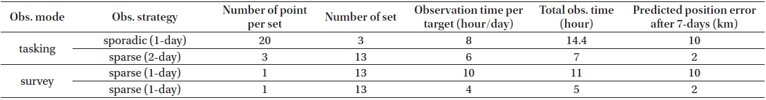
Orbit determination strategy for tasking and survey observation.
A GSO survey is needed to maintain the orbital information of cataloged objects and to detect unknown objects. When the operators of GSO satellites consider a collision avoidance maneuver, survey observation results can provide the information needed to schedule maneuver events. Four survey observation strategies (5s_1d, 5s_2d, 2s_1d, and 2s_2d) using a single optical system were simulated for the Daejeon site, South Korea.
The FOV is the most important variable for obtaining a higher detection rate. The detection rate is also related to the distribution of the inclination of GSO objects. The detection rate was also slightly increased by making more passes. The maximum detection rates for active and inactive GSO satellites were 95% and 90% with the 5s_2d system, respectively. Although the 2s_2d system yielded similar detection rate results, we selected the 5s_2d system as an optimal solution because of its higher SNR.
The precision of orbit determination for maintaining the GSO space object catalog was analyzed for tasking and survey observation. For tasking observation of 287 GSO satellites, sporadic and sparse-case observations with follow-up observation were considered. The orbital information of active GSO satellites can be maintained with 1 day of sporadic observation or a 2-day sparse observation. For inactive GSO satellites, follow-up observation 30 days after the first detection was sufficient to maintain the orbital information within 0.1° for 150 days. A long-term orbital improvement strategy was useful for inactive GSO satellite tracking. For survey observation, orbit determination for the sparse observation case was considered. We selected two observation scenarios, the 5s_2d system with three and seven elevation intervals. The orbital information of GSO satellites can be maintained at an accuracy of less than 10 km during 7 days with 30 and 15 repetitions in a 1-day observation. Further, a 2-day observation that requires more than 4 hr each day can provide suitable orbit determination accuracy for follow-up tracking.
For the development of an effective GSO survey observation, an optical tracking system requires a wide FOV (greater than 2°). Additionally, a short observation interval is needed to increase the detection rate and SNR. In this case, we simulated only systems with a 1° × 1° or 2° × 2° FOV in order to consider typical astronomical telescopes and their pixel scale. Multi-site or multi-telescope observations can reduce the risk of bad weather and overcome the limitations on the observation time. Flohrer et al. (2005) simulated a multi-site GEO survey observation of all of the cataloged objects. They found that four sites could cover all of the cataloged objects. The Optical Wide-field Patrol (OWL) team at Korea Astronomy and Space Science Institute plans to develop five optical satellite tracking sites worldwide. The OWL, an optical satellite tracking network, can be very useful for surveying the GSO region (Kim et al. 2011; Park et al. 2012).