It is well known that acceleration due to the non-sphericity of a central body can give rise to significant perturbations of the orbit of a spacecraft, especially when it is flying at lower altitudes. Therefore, applications which require accurate flight dynamics may also require the inclusion of the non-spherical terms of a central body (Cappellari et al. 1976). The acceleration due to uniform the distribution of the mass of a central body with a simple geometry typically is simply formulated. However, if a central body has a non-spherical shape with a non-symmetric mass, the acceleration can only expressed in terms of coefficients that are determined by satellite-based gravity observations. An unevenly distributed mass of a central body is usually expressed by what are known as spherical harmonic coefficients, i.e., the degree and order of the central body potential. Spherical harmonic coefficients represent the global structure and irregularities of the potential field of the central body (the gravity field of the central body); by summing up the degree and order of a special type of harmonic expansion, the central body’s gravitational potential at any point above the surface can be derived (Barthelmes 2013).

There exist many representations of the gravitational potential of a central body. Examples include spherical, spheroidal, ellipsoidal, the mass point or mass concentration, and finite element representations (Cunningham 1970). However, expressions based on spherical harmonic functions are very common (Fantino & Casotto 2009). When evaluating the gravitational potential using spherical harmonic functions, one should compute the associated Legendre functions (ALFs) and recursively evaluate them for high-degree-and-order coefficients. Bettadpur et al. (1992) reported the importance of the selection of recursive formulas during the computation of ALFs for fast processing and numerical accuracy. Indeed, older models of spherical harmonic coefficients did not consider numerical problems, as they only contained several tens of degree-and-order harmonic coefficients. However, ultra-high resolution models are very common currently, not only in models of the earth but also in the lunar gravity field due to their importance in satellite-based applications. For example, the Earth Gravitational Model 1996 (EGM96) model contains 360 degree-and-order coefficients (Lemoine et al. 1998), and a recent model covers up to 2190 degrees and orders (Pavlis et al. 2005). For the lunar gravity field, Konopliv et al. (2001) developed a series of lunar gravity models from data collected by the Lunar Prospector (LP) spacecraft up to 165 by 165 degrees and orders. Recently, a lunar gravity field model with 660 degrees and orders was announced using data provided from the Gravity Recovery and Interior Laboratory (GRAIL) mission (Konopliv et al. 2013). While processing such a high degree and order of spherical harmonic coefficients, several numerical considerations are crucial. First, the efficiency of the computing time to process ALFs recursively should be considered, as an undesirable procession time and/or a lack of storage may be encountered due to limits pertaining to numerical floating points. Second, numerical underflow and overflow with rounding errors can degrade the accuracy, which is another serious concern. Several extensive studies have been performed to optimize the performance when evaluating spherical harmonic coefficients. The most notable contributions were made by Holmes & Featherstone (2002a, b), who modified existing recursion algorithms while evaluating the partial sums of ALFs.

The Korean space program has plans to launch a lunar orbiter and lander around 2020 and also has plans to explore Mars, asteroids, and deep space in the future. Therefore, the Korean aeronautical and space science community has performed numerous related mission studies. Several preliminary design studies have already been conducted, such as an transfer trajectory analysis (Song et al. 2009, 2011; Woo et al. 2010), contact schedule analysis (Song et al. 2013, 2014), rover system design (Kim et al. 2009, Eom et al. 2012).

As the future lunar mission of Korea is one of the current interests among the Korean astronautical society, this paper focuses on the processing of a high-degree-and order lunar gravity field model. However, it is important to note that the current algorithm can be applied to any planet which has a non-spherical body shape. Applying the lunar gravity field model to the flight dynamics of a lunar orbiting satellite was initially done by Song et al. (2010) in Korea. They developed a precise lunar orbit propagator and analyzed the characteristics of the orbital decay time of a spacecraft flying near the moon. In their simulation, the LP165 gravity field model was used to compute the acceleration due to the non-sphericity of the moon. However, as no significant changes in the decay time were observed, even with more harmonic coefficients. Moreover, Song et al. (2010) did not consider degrees and orders over 50 by 50. In the work of Song et al. (2010), ALFs were processed with a conventional computing method, though such a low degree and order may not cause serious numerical problems. Nevertheless, using a lunar gravity field with higher degree-and-order characteristics with recently announced models is necessary for high-precision work.

Therefore, this work attempts to improve the performance of the earlier lunar orbit propagator developed by Song et al. (2010) and furthermore to apply it to Korea’s lunar flight dynamics subsystem (FDS), which is currently under development. An algorithm with proven efficiency when used to evaluate high-order gravitational harmonics (Holmes & Featherstone 2002a, b) is utilized in conjunction with an existing lunar orbit propagator (Song et al. 2010). The performance of the implemented algorithm is verified in comparisons of orbit prediction solutions obtained from STK/Astrogator. STK/Astrogator is the commercial software developed by Analytical Graphics, Inc. (AGI) in cooperation with the NASA Goddard Space Flight Center (GSFC) Flight Dynamics Analysis Branch (FDAB). STK/Astrogator was already used and verified its’ performance while analyzing and planning various past planetary missions. The achieved performance enhancement, in terms of both the computation time and the degree of accuracy degradation when using the current algorithm, are also analyzed in detail. In Section 2, the theory used to implement the current algorithm is discussed, with detailed algorithm flows. Simulation results including a performance validation with STK/Astrogator, the achieved performance enhancement in terms of both the computation time and the degree of accuracy degradation are shown in Section 3. Finally, conclusions are given in Section 4. As the performance of the implemented algorithm is firmly validated, it can thus be used as a basis for developing an operational FDS for the future lunar exploration mission of Korea. It can also be used to analyze various missions that require precise flight dynamics in their operation in very close proximity to the moon.

The conventional perturbing accelerations acting on a spacecraft at an external point P due to a non-spherical shape of a central body, the moon in this study, can be described by the aspherical-potential function V, as in Eq. (1) (Vallado 2013),

where r is the distance to a spacecraft from the center of the moon, φ and λ are the latitude and the longitude of a spacecraft with respect to the Moon-centered Moon mean equator and prime meridian (M-MMEPM) frame, G is the universal gravitational constant of the moon, M is the moon mass, R_M is the moon’s equatorial radius, and P_nm denotes the Legendre polynomials with degree n and order m computed from the recursion relationship. Finally, C_nm, S_nm denotes the non-normalized harmonic coefficients. The geometry of the described potential function is shown in Fig. 1.

From Fig. 1, the relationships between the spherical, P(r,φ,λ) , and the Cartesian, P(x,y,z), coordinates of external point P can easily be derived, as follows:

While processing the given harmonic coefficients using an older gravity field model with Eq. (1), numerical problems may not be serious, as these models were provided in non-normalized values with relatively low-degree-and-order harmonic coefficients. However, most current harmonic coefficients released with normalized values with having higher degree-and-order terms. For satellite applications which do not require very precise accuracy levels, evaluating harmonic coefficients with 1) remains valid. To use normalized degree-and-order harmonic coefficients with a conventional computation method, the relationships between the non-normalized and the normalized coefficients in Eq. (3) should be utilized (Vallado 2013).

Here, k=1 if m=0, and k=2 if m≠0. Also, upper bars denote that values are all fully normalized. However, in Eq. (3), it is clear that for large values of n and m , harmonic coefficients will experience overflow while Legendre polynomials show underflow, even with double the precision accuracy. Clearly this will not only degrade the computation accuracy but will also require more computational time. Thus, if fully normalized harmonic coefficients are considered, P_nm should also be fully normalized, i.e., , as expressed by Eq. (4).

The non-sectorial portion of fully normalized associated Legendre functions (fnALFs), , can be computed as follows (Colombo 1981)

The other terms in Eq. (5) are defined as shown below.

For the sectorial portion of the fnALFs, , (i.e., n= m), the recursion can be expressed Eq. (7) (Colombo, 1981); these are computed using the initial values of =1 and , where u=sinφ.

With , the recursion formulas for trigonometric functions may also combined while evaluating cos mλ and sinmλ, as in Eq. (8) (Fantino & Casotto 2009).

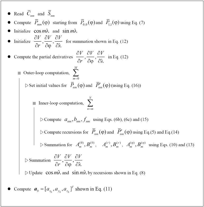
Unlike the conventional computation method described in Eq. (4), an aspherical-potential function can be rewritten with defined with “lumped coefficients,” as in Eq. (9) (Holmes & Featherstone 2002a, Fantino & Casotto 2009).

In this equation, the defined “lumped coefficients” and are given as follows (Fantino & Casotto 2009):

In Eqs. (9) and (10), M is the maximum finite degree of the spherical harmonic expansion. Here, one interesting fact is that the partial sums of fnALFs are computed in reverse order (expressed by Eqs. (9) and (10)) in the form of modifications of existing recursion algorithms (Holmes & Featherstone 2002a, b). Therefore, the loop starts by increasing the harmonic coefficient m, after which all dependent orders of the harmonic coefficient of n are evaluated. To evaluate the inner sums, Eq. (7) is used to start the polynomial recursion when m=n ; for others, Eq. (5) is used up to n=M. As discussed earlier, there are several recurrence relationships in the evaluations of the fnALPs; however, the forward column method is proven to be fast and reliable (Fantino & Casotto 2009) and is therefore used in this work. For more details on the implementation of the forward column recursion process, readers are referred to works done by Holmes & Featherstone (2002a, b).

To determine the acceleration due to the non-sphericity of a central body expressed in body-fixed Cartesian coordinates, a_b=[a_xb,a_yb,a_zb]^T, the transformation from spherical to Cartesian coordinates with partial derivatives connecting them can be derived by Eq. (2) below.

In addition, the partial derivatives of the non-spherical portion of the potential with respect to r, φ and λ can be derived as shown below (Fantino & Casotto 2009):

The lumped coefficients for the first-order partial derivatives of the potential are also determined (Fantino & Casotto 2009):

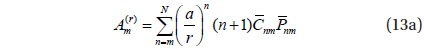
The recursion of the first derivative of the Legendre polynomial, shown in Eq. (13), is then calculated (Holmes & Featherstone 2002a),

where

For the sectorial , f_nm, and the associated fully normalized Legendre polynomial is computed as follows (Holmes & Featherstone 2002a):

If we insert the partial derivatives of the non-spherical portion of the potential with respect to r, φ and λ (shown in Eq. (12)) into Eq. (11), then a_xb, a_yb and a_zb become components of the accelerations due to the non-sphericity of the central body expressed in a body-fixed frame. However, note that the perturbing forces due to non-spherical harmonics are transformed into the inertial frame, the Moon-centered moon mean equator at the epoch J2000 (M-MME2000) frame in this study, to integrate the equations of motion numerically. The described evaluation procedure overall is depicted in Fig. 2.

As this work mainly concerns the effect of perturbing acceleration due to the non-spherical shape of the moon, the effects of other perturbing forces, such as third-body and solar radiation pressures acting on a spacecraft, are excluded from the simulation. Among the various spherical harmonic expansions of the lunar gravity field, the LP165P model, which provides 165 degrees and orders, is used in this study. JPL DE405 is used for an accurate determination of the planets’ ephemeris and for all planetary constants (Standish 1998). For numerical integration, the Runge-Kutta-Fehlberg 7-8^th order variable step size integrator is used with a truncation error tolerance of ε = 1×10^-13. Also, to convert coordinate systems between the M-MME2000 and M-MMEPM frames, the lunar orientation specified by JPL DE405 is used for high-precision work. A leap second time of thirty-three seconds is used to compute the difference between the ephemeris time and the coordinated universal time (UTC). Each simulation is done with an Intel^® Core i5 CPU, 8GB RAM, and with the Windows 8.1 Professional operating system with executable files generated from Compaq Visual Fortran. The initial epoch is assumed to be Jan-01-2018 00:00:00 (UTC) corresponding to Korea’s first experimental lunar orbiter mission, which is currently planned to be launched near around 2017~2018.

With the evaluated algorithm to compute the acceleration due to the non-sphericity of the moon, a fictitious spacecraft orbiting the moon is assumed and the orbit prediction performance is validated in comparisons with solutions obtained from STK/Astrogator. For a fictitious lunar orbiter, it is assumed that the orbiter is orbiting the moon with a circular orbit at an altitude of 100 km. Therefore, the initial orbital elements in the M-MME2000 frame are given as follows: a semi-major axis of about 1,838.2 km, zero eccentricity, right ascension of the ascending node of 0 deg and finally an argument of latitude of 0 deg. To consider various lunar surfaces that show different attractions, posi-grade, retro-grade and a polar orbit around the moon are selected while assuming the six different orbital inclinations of 0, 30, 60, 90, 120 and 150 degs. The orbit propagation duration is set to seven days in earth time, as a conventional lunar orbiter mission determines its orbit one to three times per week (Mackenzie et al. 2004; Ikeda et al. 2009). In Fig. 3, the corresponding lunar ground tracks are shown for six different orbital inclinations. It is readily apparent in Fig. 3 that wide ranges of lunar surfaces are covered with the different selected inclinations.

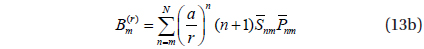
As a performance validation, orbit prediction results between STK/Astrogator and the current simulation were compared, as shown in Table 1. To compare the results, simulations are performed with a full degree and order (165 by 165) of harmonic coefficients. Also, the performances are validated by a direct comparison of the final states in the M-MME2000 frame after seven days of propagation. Final state comparisons in the inertial frame are a routine method when validating a developed FDS for use during the actual operation of any given spacecraft. Also, it is important to note that the states obtained from STK/Astrogator are assumed to be reference values; the results obtained from the current simulation are subtracted from these reference values to derive every absolute magnitude of the delta states (|Δr_x|, |Δr_y|, |Δr_z|, |Δr|, |ΔV_x|, |ΔV_y|, |ΔV_z| and |ΔV|) shown in Table 1.

As shown in Table 1, the maximum state differences between STK/Astrogator and the current simulation at the final time of the prediction were found to be approximately 83.74 cm in terms of the position and 0.82 mm/s for the velocity. Therefore, it can be concluded that every prediction result is in good agreement with the results obtained using STK/Astrogator, within 1 m or less for the position and 1 mm/s for the velocity accuracy. As the results from STK/Astrogator are assumed to be the true values, the authors believe that these performance levels are sufficiently accurate. In fact, Lunar Operational Orbit Determination Program (ILOODP) of the Indian Space Research Organization (ISRO) was validated with LP mission ephemeris obtained from NASA’s Goddard Space Flight Center (GSFC). These results were approximately 25 m and 4 cm/sec for the accuracy of the position and velocity, respectively, for a one-day prediction during the lunar mapping (LM) phase (Vighnesam et al. 2006). The results also indicate that the evaluated algorithm is well implemented, confirming that it can be applied to an operational FDS for the upcoming lunar exploration mission of Korea, especially for the phase where the spacecraft is flying in very close proximity to the moon. In addition to these results, the computation times for each of the different inclined cases are compared in Table 2. Despite the different inclinations, every simulation was completed within 5.33 min to process the given full-degree-and-order (165 by 165) gravitational harmonics, showing a mean processing time of nearly 4.36 min, which is relatively acceptable in an actual operational sense. A more detailed analysis of the processing time with respect to different degrees and orders of the spherical harmonics will be considered in the following subsection.

In this subsection, the required computing time and the resulting accuracy levels with respect to different degrees and orders of the harmonic coefficients are analyzed. In the following discussions, Method A is the result with the conventional computation method for evaluating perturbing accelerations due to spherical harmonics as adapted in Song et al. (2010). Method B is the current simulation result which utilized the forward column method with fnALFs. For a comparison of the computation times and resulting accuracy levels, the orbital inclinations of a fictitious lunar orbiter are fixed at 90 deg, with a polar orbit, and only up to 90 degrees and 90 orders of lunar spherical harmonics are compared. The main reason for limiting the degree and order levels to 90 by 90 is that the computation time with Method A required more than the actual time (i.e., it required more than a week to simulate seven days of orbit predictions), if more than 90 by 90 harmonic coefficients are applied. The required computation time between Methods A and B are compared, and the corresponding results are shown in Table 3. As expected, the overall computing time simulated with Method A required more time than Method B. However, the time differences are virtually negligible, at less than 4 sec, until the degree and order of the harmonic coefficients reach 50 by 50. If more degree-and-order harmonic coefficients are applied, the computation time differences increase remarkably, as shown in Table 3. For the 60 by 60 case, the computation time with Method A showed a time of approximately 197. 84 sec (3.30 min), and with Method B, a time of 36.30 sec (0.61 min) is required, leading to a difference of about 2.61 min. When the degree and order are 70 by 70, it was found that a time of 1,034.69 sec (17.24 min) is required with Method A. For Method B in this case, the time is 54.33 sec (0.91 min), showing an approximate difference of 16.33 min. If more degrees and orders of harmonic coefficients are computed with Method A, the required computing time reaches nearly 3.53 hours (12,685.756 sec for the 80 by 80 case) and about 18.15 hours (65,324.154 sec for the 90 by 90 case), while the processing times with Method B are still within minutes, i.e., less than 2 min (1.17 min for 80 by 80 and 1.51 min for 90 by 90). For the other higher degree-and-order cases, the computation time only with Method B was measured, with all of the results being less than 317.64 sec (5.33 min) to process the harmonic coefficients. Therefore, it is clear that the computation time differences between with Methods A and B will increase greatly when considering degree-andorder harmonic coefficients which exceed 90 by 90. Without a doubt, such a long computation time with Method A is indeed hopelessly inefficient; therefore, utilizing Method B is likely a better choice when evaluating accelerations due to the higher degree-and-order gravitational potential function, as orbit predictions play key roles in every mission-related analysis.

In addition to the computation time inefficiencies, another critical point is that the prediction accuracy levels are degraded when simulated with Method A. Therefore, the tendency of the degradation accuracy is analyzed when different orders of degree spherical harmonics are applied. To analyze the accuracy degradation, all simulation results using Methods A and B are compared to those obtained from STK/Astrogator. To compare these results, the same validation strategy shown in Table 1 (states obtained from STK/Astrogator are assumed to be reference values and the results obtained using Method A or Method B are subtracted to derive every absolute magnitude of the delta states in the M-MME2000 frame) is applied. Once again, it is important to note that the current simulation compares the results at an altitude of 100 km with a circular, polar orbit around the moon with seven days of orbit prediction. In Tables 4 and 5, orbit prediction accuracy comparison results between STK/Astrogator and the results obtained using Methods A and B, respectively, are shown.

Through a careful investigation of Table 4, it can be seen that the orbit prediction accuracy between STK/Astrogator and Method A remain at less than 10 cm for the position and less than 0.1 mm/s for the velocity magnitude until degree-and-order of spherical harmonics of 50 by 50 are applied. However, as the applied degree and order of the harmonic coefficients are increased, the differences in the predicted position states are also increased. The order of the differences reached the m level (about 16.14 m for the position magnitude) with degree-and-order harmonic coefficients of 90 by 90. The predicted velocity magnitude differences also increased, showing differences of approximately 1.43 cm/s. This velocity difference is quite large, at nearly 100 times greater than the differences observed when degree-and-order harmonic coefficients of less than 50 by 50 are applied. Also, in the results shown in Table 2, the increase in the moment of the orbit prediction difference nearly matched the moment when the required computing time starts to increase. Although these are trivial results, they confirm that an evaluation of perturbing forces due to a high-degree-and-order gravitational potential function with Method A can also lead to unexpected performance degradation during numerical simulations. In Table 5, the orbit prediction accuracy is compared between STK/Astrogator and Method B when different degrees and orders of harmonic coefficients are used. Unlike the results shown in Table 4, no serious degradation of the orbit prediction accuracy is observed in this case. Every predicted difference between STK/Astrogator and Method B as less than 22.97 cm for the position (the largest difference was noted with 70 by 70) and less than approximately 0.14 mm/s for the velocity (the largest difference arose with 60 by 60) magnitude, even when harmonic coefficients of 90 by 90 are considered. These results indicate that an evaluation of perturbing forces due to high-degree-and-order gravitational potential functions with Method B not only reduces the processing time but also guarantees the prediction accuracy. However, one may note that the prediction accuracy between Method A and B is almost identical until consideration of harmonic coefficients of 70 by 70, except the processing time. From these results, it can be concluded that numerical errors which arise during the process of evaluating ALFs can cause serious orbit prediction accuracy degradation, even when the other systemic algorithms and parameters used in simulations are identical between Methods A and B. Therefore, if orbit predictions are planned with longer prediction durations with higher degree-and-order harmonics shown in the current study, more serious computing time inefficiencies and more severe accuracy degradation may be observed.

In this paper, a proven and efficient means of evaluating perturbing forces due to higher degree-and-order gravitational harmonics due to the non-sphericity of a central body is described and implemented into a previously developed precise lunar orbit propagator. Unlike former work which used a conventional computation method, the current work adapted a well-known recursion formula that directly adapts fully normalized associated Legendre functions while processing the gravitational harmonics coefficients. This implementation is intended not only to reduce the computation time but also to prevent the accuracy degradation which can arise during numerical simulations. To validate the performance of the implemented algorithm, predicted orbit solutions are compared to solutions obtained from STK/Astrogator. Enhancements of the computation time and the accuracy degradation tendencies are also compared in the results obtained from earlier and the current work. For test cases, the orbit of a fictitious lunar orbiter is predicted for approximately seven days in earth time. It is assumed to have a circular orbit with an altitude of 100 km with various orbital inclinations. As a result of the performance validation, the differences in the predicted orbital states between STK/Astrogator and the current work were all less than 1 m for the position and 1 mm/s for the velocity accuracy, even under different orbital inclinations with full-degree-and-order gravitational coefficients (165 by 165). For a comparison of the computation time, there were no significant differences between the method applied in the previous and current work until the degree and order of the gravitational coefficients reached 50 by 50. However, a significant amount time was saved by adapting the current method with high-degree-and-order harmonic coefficients. The conventional method used in earlier work required about 18.15 hours of computing time to predict a seven-day orbit with 90 by 90 harmonic coefficients, while the time with the simulation with the current method remained within minutes, i.e., at about 5.33 min, even with coefficients of 165 by 165. For numerical accuracy comparisons, the utilizing current method matched the solutions obtained from STK/Astrogator within tens of cm for the position and within mm/s for the velocity when 90 by 90 harmonic coefficients are considered. However, the order of the predicted states increased greatly to nearly tens of m for the position and cm/s for the velocity when the previous method was utilized. Given these results, it can be concluded that both the computation time and prediction accuracy can be enhanced with the proposed method, especially when evaluating high-degree-and-order harmonic coefficients. As the performance of the implemented algorithm is firmly validated, it can be applied to the development of an operational flight dynamics subsystem for the future lunar exploration mission of Korea and to analyze various mission scenarios that require precise flight dynamics to operate in very close proximity to the moon.