Sampling discrete points from an original continuous signal unavoidably produces ambiguity of information. Known as the aliasing effect, this effect limits the utilizable bandwidth of the analog-to-digital signal conversion. As the analog signal is acquired discretely in the signal’s domain, the complete contents cannot be obtained in an accurate form. It is well known that only the slowly varying features can be correctly reconstructed from the converted digital signal according to the Nyquist-Shannon sampling theorem [1]. Higher frequencies are falsely converted down through the corresponding mixing process of signal sampling. In the resultant spectrum, they are aliased and possibly collide with the original contents of the same frequency band. In order to avoid this effect, a low-pass filter is routinely placed before an analog-to-digital converter (ADC). It is usually called an anti-aliasing (AA) filter for its function. The AA filter has been regarded as an essential element of the signal conversion.

The same principle applies to digital imaging systems by which continuously distributed information of space is sampled with a matrix of discrete photon sensors known as pixels [2-4]. The acquired digital image is the same as the original only in the slowly varying features. The aliasing effect of digital imaging is more frequently observed in color imaging systems when they employ single monolithic image sensors which have periodically arranged color pixels. Because of the lowered sampling frequency, each color component has a higher chance of the aliasing effect. It becomes the most unacceptable when fine periodic patterns of an object are acquired at good optical resolutions. By superposing its image on the pixel matrix, a kind of moiré pattern is produced, which gives a very unrealistic and perceptively annoying sense to the human viewer. In the fields of digital imaging applications, the aliasing effect acts as a deterministic noise source with the incorrectly reconstructed dataset. This has serious impact when quantitative properties are to be extracted from the acquired image data through linear or nonlinear post-processing schemes. For example, accurate evaluation of the object’s color may be hindered by the aliased components when a digital color camera is utilized for inspecting a finely structured object in applications such as machine vision or biomedical diagnosis [5, 6]. One must note that the aliased false signal, once acquired, cannot be removed by the post-processing schemes. It must be rejected at the stage of the image acquisition by an optical means.

An optical AA filter is a low-pass filter that acts on the 2-dimensional image information. It is usually equipped on the image sensor package to scatter the light fields in controlled manners [2, 7, 8]. It introduces a slight blur of the image contents to remove the fast varying features before being acquired. In this principle, the AA filter can be implemented by various methods. Polarization-sensitive beam splitting is one of the most popular schemes while any light diffusing elements can be used for the same purpose. Some of the AA filter implementation methods may provide operational flexibility [7-9]. Their filter characteristics are freely adjusted by the users. The optomechanical AA filter is a recently introduced method that supports such an adjustability for the users’s preference [9]. In this implementation of the AA filter, the relative position of pixels to the image mechanically dithers to make an engineered motion blur. The intended blur directly gives a low-pass filter effect. By the active mechanism, the optomechanical AA filter can be adjusted by the mechanical dithers and, of course, can be turned off to make no effect on the image.

In general, the performance of an AA filter is quantitatively measured by the optical transfer function (OTF) in the spatial frequency domain, or its modulus of the magnitude transfer function (MTF) [10, 11]. The idealized AA filter completely rejects all the signal components above the Nyquist frequency while preserving well the low-frequency components. Hence, the magnitude of the OTF, i.e. the MTF, must be zero in the stop band while it must be unity in the pass band, making a flat-top curve in its transfer characteristic. For the conventional intensity-sensitive imaging with the incoherent light fields, the conventional OTF is given as the transfer of the signal intensities, rather than that of the fields directly [11]. It suggests that the design freedom of the AA filter is insufficient for making an ideal flat-top filter. Multi-pole filter design strategies, which have been useful in electrical filter designs, are not applicable. A realizable AA filter must always exhibit a considerable signal loss for the pass band or an imperfect rejection for the stop band. By the loss, the AA filter is often blamed for degrading the image acuity and sharpness, particularly when the image sensor has a limited number of pixels. In the opposite side, an AA filter can be unacceptable by the insufficiently suppressed aliased components when very little error is expected for quantitative image analysis. This dilemma needs to be resolved for the optical AA filter.

The optomechanical AA filter is an attractive image-filtering scheme. It utilizes mechanical actuators that vibrate the image sensor or the objective lens in the transverse plane during the photon integration time. Owing to popularity of the optical image stabilization (OIS) technology, this type of AA filter can be implemented at minimum cost. An OIS-equipped camera has internal actuators for compensation of the camera’s motion in a shot, which can be used simultaneously for the AA filtering [12]. By taking advantage of this convenience, a Japanese camera maker, Pentax of Ricoh Imaging Co., recently commercialized a digital single-lens reflex (DSLR) camera, K-3, with an optomechanical AA filter [9]. A very useful feature is found in its adjust-ability. The user can freely turn the AA function off for ordinary objects that make only slight visible moirè patterns. One more advantage which has not been emphasized yet can be found in its greater freedom of filter design. In the optomechanical AA filter, the point-spread function (PSF) of the filter can be directly tailored by the actuation protocol to provide an optimal MTF.

In this research, we have investigated the optimal design of the optomechanical AA filter which can effectively remove the aliasing effect of the digital color camera. Instead of using the circular motion introduced earlier by Pentax [9], we developed a spiral motion protocol which can make Gaussian-like PSF and MTF characteristics. We observed that our deliberate design of the optomechanical dithers greatly improves the high-frequency suppression. We also found that the pass band characteristic can be enhanced by a color-differential acquisition which is a unique advantage of the optomechanical AA filter. We successfully demonstrated a digital imaging scheme of little aliasing effect and minimum loss of image acuity by this method.

The aliasing effect in the digital color imaging is to be overviewed in this section for complete understanding of our AA filter scheme.

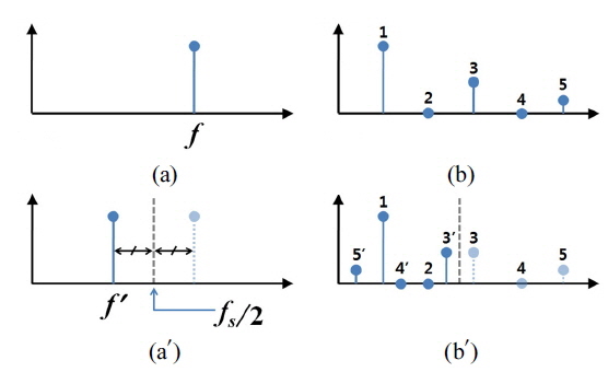
In a typical signal conversion, a continuous signal is sampled by a series of signal detections given periodically at a rate of the sampling frequency, f_s. The converted discrete signal defines a finite bandwidth of zero frequency to the maximum extent of f_s/2, called the Nyquist rate. Note that the discrete signal can only be defined in the base band by the discrete Fourier transformation. The sampling process can be described by mixing the raw signal with a pulse train of detection. In the frequency-domain picture, its spectrum takes an operation of the integral convolution with a frequency comb that corresponds to the serial sampling action. The aliasing effect is easily explained by the resultant signal spectrum which is packed in the base band. The signal conversion makes an effect of folding the spectrum, possibly inducing overlapped spectra in the base band. Figure 1 shows the frequency-domain pictures of the raw signals [(a) and (b)] and those of their converted forms [(a′) and (b′)]. The vertical dashed lines indicate the Nyquist frequency. For a high-frequency component of frequency f, shown in Fig. 1(a), its converted spectrum has its signal at a different frequency, f′ as shown in Fig. 1(a′). The aliased component at f′ forms a mirror image of the original with reference to the Nyquist frequency. For multi-component signals as in Fig. 1(b) and (b′), each signal component is aliased independently in the converted spectrum. Ambiguity may arise between the aliased and the original in the same band. Notice that, throughout this report, a spectrum primarily means the Fourier conjugate of a spatial image signal in the reciprocal domain of space.

Digital imaging is different from a simple analog-to-digital conversion for its two-dimensional (2D) and areal sampling nature. In digital imaging, the signal conversion to a discrete form is carried out through a pixilation process. Because of the 2D property, two spatial frequencies of f_x and f_y are needed to represent its spectrum. Here, f_x and f_y are the reciprocal domains of the spatial coordinates, x and y, respectively. As well as its temporal integration of photons, a pixel spatially integrates the incident photons with its photodetection area. By the non-point nature, the converted signal cannot be said to be sampled at points. In an averaged sense, the photodetection area must play a role of a low-pass filter by the spatial uncertainty of the detected photons. If the image sensor has a microlens array for enhancing the photon collection efficiency, the aperture of an individual lens will provide the effective detection area [13]. The aliasing effect is not concerned with very high frequencies because they are automatically rejected by those areal sampling effects as well as by the optically induced blur of the objective optics.

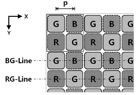
The most popular type of digital color imaging sensors utilizes the Bayer color filter array (CFA) to obtain three color channels with a single sensor chip [14, 15]. Figure 2 shows the typical arrangement of color pixels in the Bayer CFA. In Fig. 2, the boxes of R, G and B stand for pixels of red-, green- and blue-sensitive photodetectors, respectively. In every group of 2×2 pixels, two G-pixels are arranged diagonally while R- and B-pixels are put in the other two pixels. The pixel pitch, denoted by p, is defined by the distance between the neighboring color pixels measured in an axis. In this report, x and y will represent the two rectangular axes of the pixel arrangements. The green channel has two times higher a pixel density, which is advantageous for higher sensitivity of the human vision to the green light. As a consequence, the red and blue channels become more vulnerable to the aliasing effect. One more factor to be taken into account is the lower ratio of the effective detection areas that the R- and B-pixels have. It minimizes the intrinsic filter effect of the spatial photon collection. Those factors explain well why the aliasing effect mostly generates colored pattern errors of red and blue in the usual digital color imaging that employs the Bayer CFA.

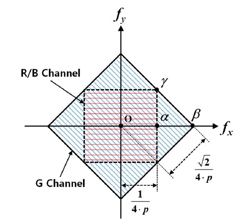
Due to the color pixel arrangement, the aliasing effect is more complicated in digital color imaging [2]. The sampling frequency differs by the color channel. The Nyquist frequency must be carefully defined for each color channel. Figure 3 shows the 2D spectral map of the Bayer CFA-based color image signals. For the red or blue (R/B) channel, the sampling interval equals to 2⋅p, arranged along x and y axes. Thus, the base band of the acquired signal, i.e. the Fourier-domain representation of the discrete signal, forms a square area aligned to the axes of f_x and f_y as shown in Fig. 3. For the green channel, however, the sampling points are aligned diagonally with an interval equal to (2)^1/2⋅p, making a wider base band area due to the doubled pixel density. The base band of the green channel forms a square area inclined by 45° as shown in Fig. 3. The aliasing effect occurs to signal components located out of the square area for each independent color channel.

The Bayer CFA-based image sensor acquires a 2D image of spatially encoded color, called color mosaic. The full color image must be reconstructed by taking a linear or nonlinear image processing scheme [14, 15]. It is basically a data interpolation task, called as demosaicking of color images. Along with simple bilinear and bicubic interpolations, various advanced algorithms such as the gradient-corrected bilinear interpolation (GCBI) have become popular for enhanced performance in acuity and signal-to-noise ratio (SNR) [14, 15]. Therefore, the final digital image is obtained through optical, optoelectronical and digital processes. It must be noted that each stage of the image formation may exhibit a filtering or filter-like effect. Because of the shift-dependent variance that comes from the finite photodetection area of a pixel and the possible nonlinearity involved with the demosaicking algorithm, the image formation cannot be preferably expressed by a linear shift-invariant (LSI) system analysis [10]. Nevertheless, one can approximate that the spatial photon collection and the data interpolation give effects similar to low-pass filtering in the averaged sense. All of those effects contribute to the final signal acquired by a color imaging system.

In this research, we investigated an optomechanical AA filter that provides better anti-aliasing performance. To make an optimal AA filter, we developed a filter design method that utilizes a spiral-motion protocol. The PSF of the imaging system, hence, is not fully determined by the optical elements but additionally tailored by the filter’s motion. Here, the optically defined PSF of the system is given by G(x,y) as a function of space. The effective PSF denoted by G_eff(x,y) defines the image of an object point actually projected onto the image sensor under dither motion. By use of the optomechanical filter, it is blurred spatially as

where ⊗ denotes the conventional integral convolution operation, and I(x, y) is the PSF of the filter motion. The function of I(x, y) defines how the optical energy is spread on the sensor plane by the relative motion. In our experiment, two actuation axes of x and y were driven by two sinusoidal driving signals with a phase difference of 90 degree. The x and y driving signals are given, respectively, by

where A(t) is the amplitude function of time t, and T_s is the period of the sinusoidal filter’s dithers. By the amplitude modulation, a spiral motion can be obtained for a desired PSF.

The filter’s response of I(x, y) can be designed by the amplitude function in our AA filter. In the approximation of the slowly varying function of A(t), a spiral actuation trajectory consists of densely assigned coaxial circle-like curves called circlets. The radius of each circlet, r, is given by r=k⋅A(t) where k is the actuation coefficient. Let us assume that A(t) is a monotonically increasing function from zero to the peak. It has its own period of T by which the spiral is completed. Within the period, we can define the inverse function of A(t) as

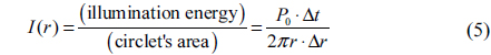
to be a function of r, which is also a monotonically increasing function. For a constant power P₀ of the image’s illumination onto the sensor plane, the filter’s PSF is found by

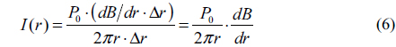
for a circular band of width Δr drawn in time interval Δt. By the property of B(r) from Eq. (4), we found a relation of

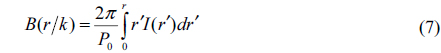
which explicitly relates the amplitude modulation to the motion-induced PSF. The inverse relation was, thus, calculated by

which is the very design formula for producing a targeted PSF of I(r). Obtained from Eq. (4) and (7), the actual amplitude function of the driving signals can be made by repeating A(t) in time with the period, T. Alternatively, it can be made by alternating the forward- and the backward-running functions of A(t) and A(T−t) periodically. For the latter case, the rapid return to the origin at the end of a spiral is avoided. In our experimental studies, this type of amplitude function was utilized for the actual driving signals.

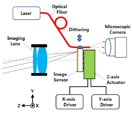
An experimental setup was constructed to study the optomechanical AA filter in a digital color imaging system. Figure 4 shows the schematic diagram of our experiment setup. A color image sensor was mounted on a 2-axis piezo-electric actuator which was driven by two electric signal generators operated synchronously. Each generated a sine signal in amplitude modulation as Eq. (2) and (3) suggested. The image sensor was mechanically dithered by the actuator on the image plane to get the desired motion blurs. A photographic objective lens was placed in front of the image sensor. The image of a test object was acquired while the image sensor was dithering. The raw image data were recorded by a computer in the form of color mosaics with no demosaicking interpolation applied. Separately, a microscopic camera was set up to monitor the in-plane dither motion of the sensor. A fiber-optic illuminator was attached on a side of the image sensor. The microscopic camera could capture the image of the fiber core under motion while the optomechanical filter was operating. This microscopic image could be interpreted as the PSF of the filter motion. In our setup, the color image sensor was a low-cost CMOS image sensor based on the color pixels of the Bayer CFA. It was equipped with 1280×1024 pixels covered by micro-lenses on the top with a pixel pitch of p = 3.6 μm in the standard 1/3-inch format. Our objective lens had a fixed focal length of 12 mm with an aperture size of f/1.4. It supported 28° for the full FOV (field of view) in the diagonal axis.

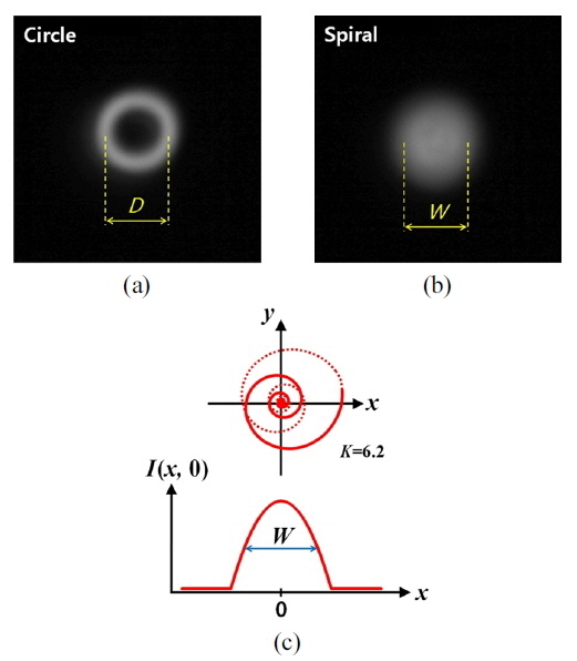
For our optomechanical AA filter, the actuator was operated by two different filter motion protocols: circular and spiral motions. Its contribution to the effective PSF could be evaluated by directly measuring the PSF of the filter, I(x,y) by the monitoring microscopic camera. Figure 5 shows the microscopic pictures of the circular (a) and the spiral filter motion (b), captured by the microscopic camera, which could be interpreted as the measured PSFs. Figure 5(c) gives a schematic illustration of the spiral trajectory and the consequent intensity distribution. In the circular motion protocol, the two axes were simply driven at a constant amplitude in drawing a circle of diameter D. Each circle was drawn in every period of T_s with no modulation. On the other hand, in the spiral motion protocol, the actuator was driven by modulated signals that changed the radius continuously in time. The amplitude function of the driving signals was made by alternating the forward- and backward-running functions as described earlier. As schematically depicted in Fig. 5(c), the spiral trajectory was drawn twice in a period of the amplitude function, that is denoted by T_a, by drawing outwards and inwards. Here, the number of circlets drawn in a period was measured by a spiral factor of K that equals to T_a/T_s. For a sufficiently large value of K, the intensity distribution that the spiral motion produced became practically symmetric. For a moderate value, one can still approximate its PSF to a continuous symmetric function due to the other contributions of optical or non-optical blurs to the final effective PSF.

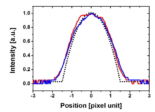
In our optomechanical AA filter, a Gaussian-like PSF is preferred for its excellent suppression of the high-frequency components. An exact Gaussian function, however, has long tails outside the central region sacrificing the time efficiency. An alternative design of the quadratic function was used in this research. It is also known as the Welch window function in the field of Fourier analysis. We designed the filter motion to produce a quadratic PSF as shown in Fig. 5(c) by using the design formula of Eq. (7). The intensity distribution of the quadratic function was specified by the width, W, defined by the full width at half maximum (FWHM) of the filter’s PSF. Driving the actuator in modulation for the quadratic function, the PSF was measured by the microscopic camera as shown in Fig. 5(b). Figure 6 shows the sectional profiles of the measured PSF (solid lines) along x and y axes. The dotted line in the figure is a quadratic function of the design target. For spatial dimensions of PSF, we will use a pixel unit that equals a pixel pitch of the image sensor. The successful result of Fig. 6 suggested that we could freely design the PSF of the filter in the spiral motion protocol with the derived design formula of Eq. (7). By adjusting the width of the PSF, the effect of the AA filter could be controlled with ease for an optimized performance.

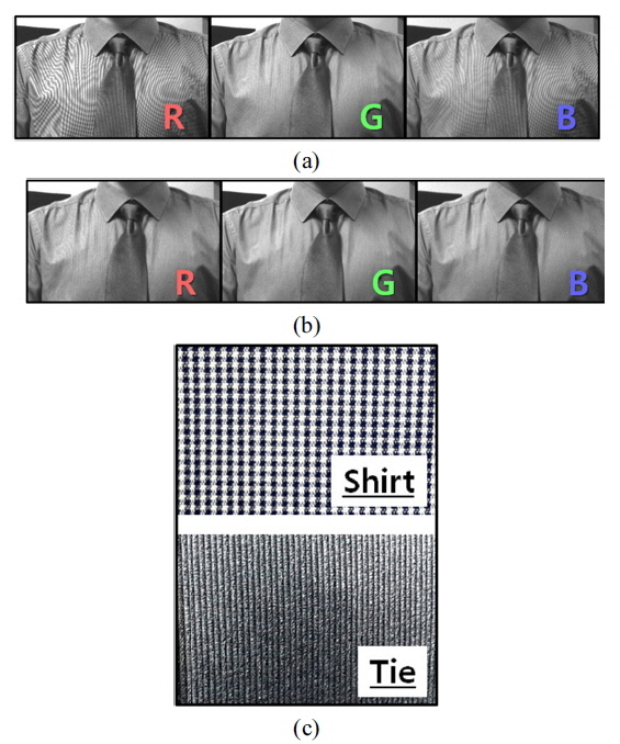
In our preliminary imaging tests, our system acquired some pictures of finely textured objects while its optomechanical AA filter was switched on and off. Figure 7 shows the digital color image acquired with no filter (a), one acquired with a spiral filter motion (b) and the close shots of the textures on the shirts and the tie of the object (c). In the presentation of the color images, each color image was separated into three color channels of R, G and B, displayed individually in gray scale. The R and B channels were prone to producing clear moiré patterns as seen in Fig. 7(a). Strange colored patterns irrelevant to the object’s texture could be observed in the final digital images. On the other hand, they completely disappeared as the optomechanical AA filter was operating by the optomechanically induced motion blurs. The imaging test also suggested that the optomechanical AA filter brought a considerable loss of acuity, perceivably received at the object’s boundaries when magnified.

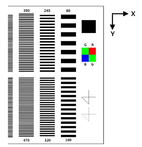
In our experiment, the image transfer characteristics of our optomechanical AA filter were quantitatively analyzed, and the suppression of the aliasing effect was evaluated as well as the signal loss of the base band. For this purpose, a resolution target was prepared in which periodic stripe patterns of multiple spatial frequencies were arranged side by side. The responses of our color imaging system were recorded for three color channels. Through the MTF analysis, the imaging characteristic was evaluated as a function of spatial frequency. Figure 8 shows the resolution target used in this study. Only a part of the target is shown in Fig. 8. It consists of 14 rectangular blocks of different spatial frequencies. In each block, black and white stripes alternated periodically in a duty ratio of 50%. Under a uniform illumination, the target located ~2 meters apart was imaged by our imaging system as described with Fig. 4. The raw image data were sent to a computer for further analysis. The amplitude of the fundamental signal component that each block produced was obtained from the captured digital image. The signal magnitude given as a function of frequency was interpreted as the effective MTF of the system. Neglecting the other sources of blurs, the optomechanical filter motion was regarded as the main contributor that dominantly determined the MTF of the system.

As described earlier, an aliased signal component appears at a frequency different from the original in the acquired digital image’s spectrum. Due to the deterministic nature of the aliasing effect explained with Fig. 1, the aliased frequency can be easily predicted from the known original frequency. Each block of the resolution target shown in Fig. 8 made a square-wave signal along the y axis, producing multiple harmonics in its signal contents. When the signal is composed of multiple harmonics, the fundamental component, i.e. the first-order harmonic is presumably dominant. If the fundamental frequency were above the Nyquist frequency, the intrinsic low-pass filtering effect of the finite pixel area would effectively reject the high-order harmonics in the acquired signal. Hence, the amplitude of the fundamental could be accurately measured in the aliased image signal with minimum interference of the other harmonic components. In our extended MTF analysis, the response of the system to an inputted signal was measured at the aliased frequency. It could quantify the magnitude of the aliasing effect, simultaneously measuring the MTF of the AA filter in an extended frequency range.

The extended MTF for the aliasing effect analysis was obtained by the procedure that follows. (I) A digital color image was taken by the imaging system with the resolution target. (II) The raw dataset of color mosaic directly obtained from the sensor was decomposed into three independent monochrome images of R, G and B channels. For the red and blue channels, the size of images became 640×480 pixels. For the green channel, the full-size image of 1280×1024 pixels was reconstructed by borrowing the pixel values from the nearest neighborhood in the x axis. (III) In a monochrome image of the resolution target, each block was segmented. The intensity function along the vertical y axis was extracted from each block. (IV) The intensity was transformed by the fast Fourier transform (FFT) algorithm. The magnitude function was obtained by absolutizing the complex spectrum obtained this way. (V) In the magnitude spectrum, the fundamental signal component was searched. It could be characterized by an intense peak at the original frequency or the aliased frequency. (VI) The final extended MTF was constructed by plotting the magnitudes versus the original frequencies for the measured fundamental components. The magnitudes were normalized so that the zero-frequency component has a unity response in the MTF. One must notice that our extended MTF is defined in an extended frequency range regardless of the aliasing effect by reassigning the frequencies in the MTF spectrum. The strength of the aliasing effect is quantified as a function of the contributor’s frequency.

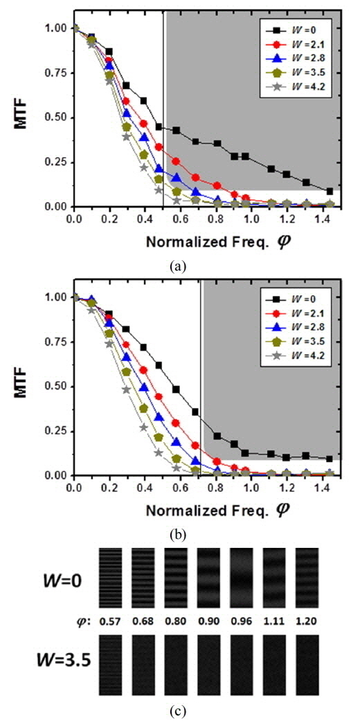
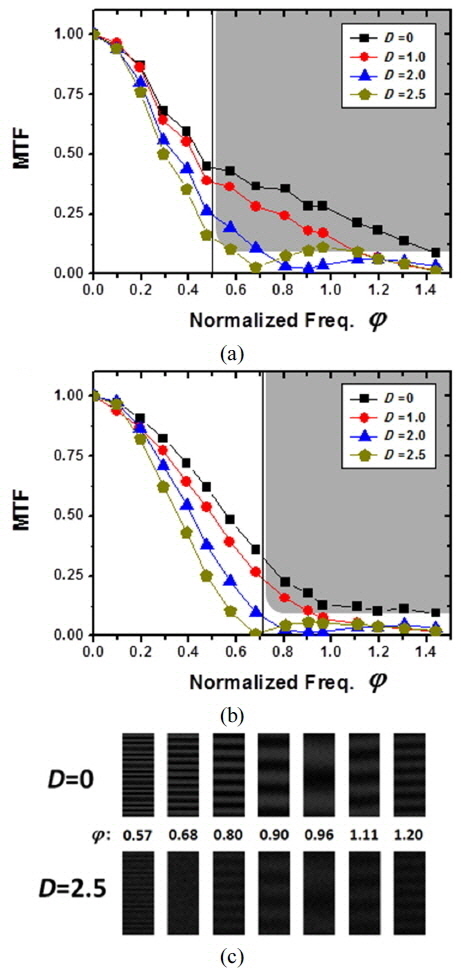
The effect of our optomechanical AA filter was analyzed by the extended MTF. The performance of the filter motion protocols could be quantitatively compared. At first, the circular filter motion protocol was given. Figure 9 shows the extended MTF of the red-channel image (a) and that of the green-channel image (b) with various diameters of the circular motion. The horizontal axis of the normalized spatial frequency, denoted by φ, corresponds to the spatial frequencies normalized by (2p)⁻¹. Figure 9(c) shows the stripe patterns of φ=0.57, 0.68, 0.80, 0.90, 0.96, 1.11 and 1.20 acquired through the red channel of the camera under the circular filter motion with D=0, i.e. no filter motion (upper row), and D=2.5 pixel units (lower row), respectively. Note that the contrast was enhanced in Fig. 9(c) for better visibility. The data depicted in Fig. 9(a) and (b) were all obtained from the stripe patterns of the target acquired as Fig. 9(c).

For the red and blue channels, the Nyquist frequency was found at φ = 0.5. Consequently, the patterns observed in Fig. 9(c) must have been generated by the aliasing effect because φ > 0.5 holds for them. Their amplitudes depicted in Fig. 9(a) were not negligible, making non-zero MTFs. In the green channel, the base band bounded by the Nyquist frequencies was tilted as explained with Fig. 3. The Nyquist frequency along the measurement axis (y axis) is, hence, doubled in effect. However, notice that it is reasonable to take for the green channel’s Nyquist frequency considering the worst cases.

The results of Fig. 9 demonstrated that the aliasing effect was reduced by increasing the diameter D. However, it eventually increased again at high frequencies as D exceeded 2.0 since the central hole of the enlarged PSF got expanded. The optimum diameter was found around D≈2.0 pixel units, still allowing weak but non-negligible aliasing effect in a wide frequency range. We observed that the aliased pattern becomes clearly noticeable when the amplitude exceeds 0.1 (10%) in the MTF. The shadowed regions in Fig. 9(a) and (b) correspond to the area of visible aliasing effect. Noticeable aliasing effects were always brought in the red channel by the circular filter motion as observed in Fig. 9(a).

For the spiral filter motion, the extended MTF was measured in the same way with various widths of the PSFs. Figure 10 shows the extended MTF of the red-channel image (a) and that of the green-channel image (b) with various widths of the spiral filter motion. The driving parameters were T_s=10 ms, T_a=50 ms and K=5 for the spiral filter. The integration time of the image sensor was 50 ms. Figure 10(c) shows the stripe patterns of φ=0.57, 0.68, 0.80, 0.90, 0.96, 1.11 and 1.20 which were acquired through the red channel of the camera under the spiral filter motion with W=0, i.e. no filter motion (upper row), and W=3.5 pixel units (lower row), respectively. Note that the contrast was enhanced for better visibility at the same degree of Fig. 9(c). Thus, the aliasing suppression performance of the spiral filter can be compared to that of the circular one, with Fig. 9(c) and Fig. 10(c), along with their extended MTFs.

The results of Fig. 10 showed that the high-frequency components were well suppressed when W > 3.0 pixel units. Even with a moderate filtering of W = 2.8, the overall high-frequency rejection performance of the spiral was better than those of the circular, comparing the results of Fig. 9 and Fig. 10. For W > 4.0, no considerable aliasing was observed in the entire frequency range, which must be preferred when no imaging error is required. The Gaussian-like PSF produced by the spiral motion must have rejected the aliasing effect in the full range. A regime of W=3~4 seems optimal for most imaging applications where the AA performance and spatial resolution must be compromised. The aliased components in the right vicinity of the Nyquist frequency have little chance to be excited thinking of the narrow area occupied in the frequency-domain representation as given in Fig. 3. Thus, the AA filter of W = 3.5 pixel units can be an optimal choice for most photographic applications. For sure, one can carefully optimize the filter performance by defining a merit function based on the data given by the extended MTF. The best compromise is a matter of engineering choice depending on the nature of the application.

Concerning the acuity of the acquired image, any type of AA filter was found to exhibit a signal loss of the base band. This issue is more serious for the green channel because its base band is two times larger by the higher pixel density. For the case of W = 3.5, nearly half of the signal energy was lost in the base band as seen in Fig. 10(b). The green channel’s acuity loss could be said to be excessive. A fact to be noted is that the green channel contributes more to the perceived luminescence, more critically affecting the perceptually visual acuity. When the number of available pixels is limited, e.g. for the case of most video cameras, such an excessive loss of the green channel’s acuity becomes more apparent in the displayed images.

To cope with the acuity loss of the green channel, we developed an interesting image acquisition protocol cooperating with the optomechanical filter. Note that the photon integration time is another design parameter in our optomechanical filter when driven by the spiral filter motion. By reducing the integration time of the image sensor below the filter’s drawing time of T_a, the PSF of the filter is narrowed from the original one. If the image sensor supports the ability to control the integration time for each of the color channels individually, a synchronized motion of the filter will provide a color-differential filtering capability. With a minimum exposure of the green light, then, the PSF of the green channel can be sharpened at an acceptable sacrifice of SNR.

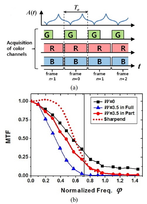
Figure 11 shows the timing chart of the color-differential filtering and image acquisition (a), the measured MTF of the green channel (b). In our color-differential filtering scheme, the green channel had a shortened integration time and its timing matched the amplitude function of A(t) as described in Fig. 11(a). The time slot of photon integration was centered at the lower peak of A(t) so that it acquires the image photons during an interval of small circlet radii. This made the PSF of the green channel much narrower because the optomechanical filter did not complete the spiral trajectory as initially designed. Yet, no commercial image sensor supports such a useful function for differentiating the color channel’s exposure. In our experiment, we mimicked the differential exposure by acquiring two images of the same scene at two different integration times. Those images were combined to a single frame by taking the green channel from the one of a shorter integration time but taking the red and blue channels from the one of a longer exposure. The final color image was reconstructed by the GCBI demosaicking algorithm.

The experimental condition of the color-differential filtering was the same with those of the simple spiral filter experiment described with Fig. 10. The only difference was made by selectively reducing the integration time of the green channel to 25 ms, 50% of the red and blue channels. The improved acuity of our color-differential filtering method was quantitatively evaluated by the MTF analysis. Figure 11(b) shows the results of the green channel’s for comparison. The case of W = 3.5 pixel units in full integration of 50 ms (triangular dots) produced an excessively reduced pass-band transfer. On the other hand, the case of W = 3.5 in partial integration of 25 ms (circular dots) exhibited an enhanced MTF because of the effectively reduced width of the spiral motion. Still, the high-frequency components were well suppressed for a reduced effect of aliasing. Notice that our color-differential acquisition gave no effect to the red and blue channels.

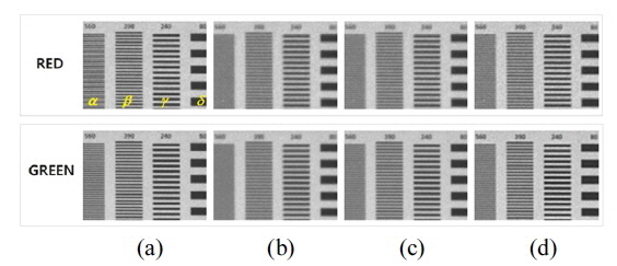
The digital filtering could further enhance the MTF with little concern of the aliasing errors once suppressed by the AA filter. A high-frequency boosting filter, also known as a sharpening filter, could be used to amplify the high-frequency components. Note that such a digital filter could amplify the aliasing effect, if not properly suppressed by an AA filter. In our post-processing image enhancement, a finite impulse response (FIR) filter of image sharpening was applied to the image acquired by the color-differential filtering. Figure 12 shows the partial images of the resolution target obtained from the raw data in no filter operation (a), those of the spiral filter, W = 3.5 and K = 5, in full integration (b), those of the color-differential spiral filter with a green channel of 50% exposure (c), and the images of the color-differential filter which were sharpened by the digital FIR filter (d). In Fig 12, the color images reconstructed by the GCBI are displayed with separated color channels (red and green) in gray scale.

Inside each image of Fig. 12, four blocks of black and white stripes are shown, named as α, β, γ and δ from the left to the right. The normalized frequencies of the blocks were 0.683, 0.476, 0.293 and 0.098, respectively. The aliasing effect was clearly observed at the red channel of α in Fig. 12(a) when no AA filtering was given. It disappeared after applying the optomechanical AA filter as in Fig. 12(b), (c) and (d). The acuity of stripes decreased as a consequence as in Fig. 12(b). It was particularly obvious for the green channel of β in Fig. 12(b). Even though its frequency was φ=0.476, well below the Nyquist frequency, the contrast was very weak and could not be clearly resolved. This signal was saved by the color-differential filtering and further amplified by the sharpening filter. In the final image of the green channel, Fig. 12(d), the overall acuity loss became small compared to Fig. 12(a).

The reduced acuity loss of the color-differential filtering scheme was also confirmed by the MTF analysis given by Fig. 11(b). The color-differential filtering after the digital sharpening (dotted line) was compared to the AA filter response of full integration (triangular dots on a solid line). The intermediate frequency range of φ = 0.4~0.6 was found to be boosted by a factor higher than two while maintaining negligible amplitudes of the aliasing effect in φ > 0.71. Those experimental results verified that the benefit of our optomechanical AA filter in the suppression of the aliasing effect could be obtained with a little sacrifice of the resolutions when cooperating with the color-differential filtering scheme and the digital post-processing method. Our optomechanical AA filter with a spiral filter motion was found to provide a better compromise between the aliasing suppression and the resolution performance by utilizing the color-differential acquisition scheme. This advantage has not been achieved by any other AA filter types.

In this research, we investigated the AA filtering method based on the optomechanical dithering element. By the spiral motion protocol, a very useful filter design strategy was established in this study. In principle, any physically allowed design of the AA filter can be implemented by designing the AA filter motion. We experimentally confirmed that our optomechanical AA filter can provide an excellent filtering power with a better compromise of the AA performance and the signal loss. In this study, we developed a filter design formula and the extended MTF analysis for quantitative evaluation of the AA filter characteristics. We believe that our AA filter can be useful in low-error imaging measurement technologies which require integrity of image data for further quantitative analysis. As well, it can be utilized for ordinary photographic applications such as video capturing where annoying moiré patterns must be suppressed.