With the development of astronomical optics, space optics [1-3] and inertial confinement fusion, large-aperture optical systems have been widely used. For very large optical elements, however, the aperture may be too large for the interferometer to test in one pass. In 1982, C. J. Kim solved this problem with the sub-aperture stitching method [4]. However, location errors are inevitable with this method. Thus, researchers use overlapping areas between the sub-apertures to compensate for location errors [5-9] such as piston, tilt, defocus, clocking, and position errors. In most cases, only piston, tilt, and defocus errors are corrected. For large optical elements which are tested by many sub-apertures, it takes much time for a sub-aperture stitching algorithm to get the stitching result. To quickly compensate for piston, tilt, and defocus errors, we develop a fast algorithm, which is easy to understand and program.
In Section 2, we briefly introduce our algorithm. In Section 3, we compare the time complexity of our algorithm with the current algorithm. In Section 4, we study the accuracy of our algorithm using simulation. In Section 5, we discuss an experimental result demonstrating the effectiveness of the proposed algorithm. Finally, we present our conclusions in Section 6.
II. FAST ALGORITHM FOR SUB-APERTURE STITCHING
The current algorithm uses a least-squares method to remove relative piston, tilt and defocus errors directly. In our algorithm, we calculate the partial derivative of data before using a least-squares method to remove relative piston, tilt and defocus errors. The reason for calculating the partial derivative of data is that it makes the least-squares method much easier. Actually, using the least-squares method after calculating the partial derivative of data is just averaging, so it makes the algorithm faster than current algorithm.
For convenience, we only discuss the testing of spherical optical elements in this article; however, with some modifications, this algorithm can be easily applied to the testing of both flat and aspheric optical elements.
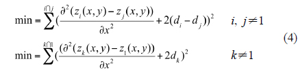
One sub-aperture, usually the center sub-aperture, is selected as the reference sub-aperture. The remaining sub-apertures have nonzero piston, tilt, and defocus errors that are relative to the reference sub-aperture. Thus, we compensate for relative piston, tilt and defocus errors [9] as follows:

where
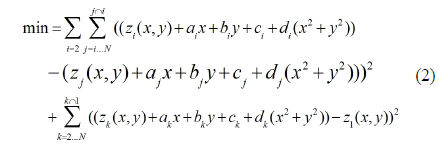
Assuming that there are N sub-apertures and that the reference sub-aperture is number 1, current sub-aperture stitching algorithms use the least-squares method to directly calculate the necessary compensations [5-9]:
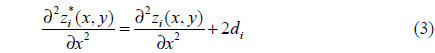
In our algorithm, we first calculate the second-order partial derivative of Equation 1 with respect to the independent variable x:
Then, we use the least-squares method to calculate the needed compensation between two adjacent sub-apertures:

Solving Equation 4, we obtain the following over-determined linear equations:
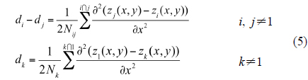
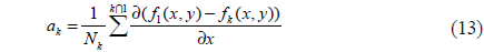
As we can see, using a least-squares method after calculating the partial derivative of data is just averaging. Here, Nij is the total number of pixels in the overlapping area of the i-th sub-aperture and the j-th sub-aperture, and Nk is the total number of pixels in the overlapping area of 1-st sub-aperture and k-th sub-aperture.
We can easily use the weighted least-squares method to solve the over-determined linear equations by setting the weight equal to the total number of pixels in the corresponding overlapping area.
Using the calculated coefficients of the relative defocus, we compensate the defocus errors:

where

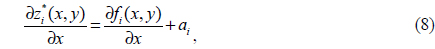
To compensate for the relative tilt errors, we calculate the first-order partial derivative of Equation 7 with respect to independent variable x and the independent variable y:

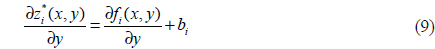
We use a similar procedure to calculate

where
Finally, we use the same method to compensate for the piston errors and stitch the resulting measurement data to obtain a full-aperture result.
III. TIME COMPLEXITY OF THE ALGORITHM
In this section, we assume that there are only two sub-apertures, where one sub-aperture is the reference sub-aperture, and the overlapping area is a square (n × n pixels).
In the algorithm currently in use, Equation 2 leads to linear equations:
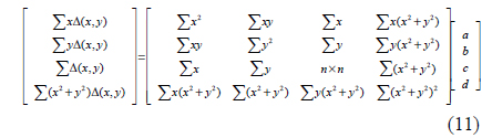
where ∆(
Solving Equation 11, we obtain the coefficients
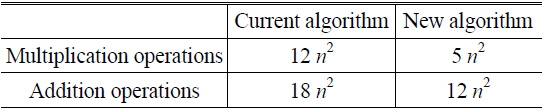
Time complexity
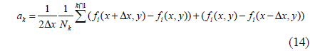
In our new algorithm, we use differences to calculate partial derivatives. For instance, we find the first-order partial derivative using

where ∆
we calculate it using

Thus, we use about 5
In Table 1, we can see that our algorithm has a much lower time complexity than the current algorithm.
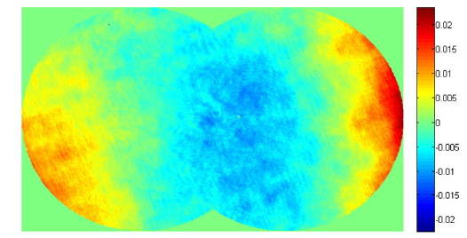
In the simulation, a measurement result (501 × 801 pixels, shown in Fig. 1) was first divided into two sub-apertures. After dividing the measurement result into sub-apertures, we add random noise ([-0.001, 0.001] wavelength) and piston, tilt, and defocus errors to each sub-aperture. We use both the current algorithm and the new algorithm to calculate the compensators. We repeated the simulation calculations 20 times. In all 20 simulations, the accuracy of the new algorithm is lower than that of the current algorithm. We present one typical result in Table 2.
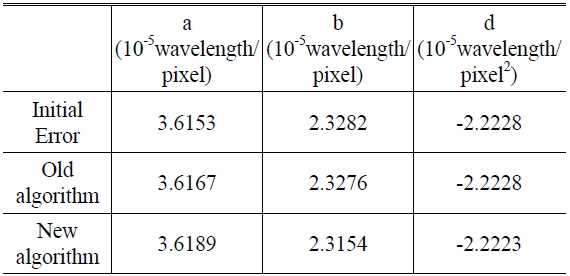
Simulation results
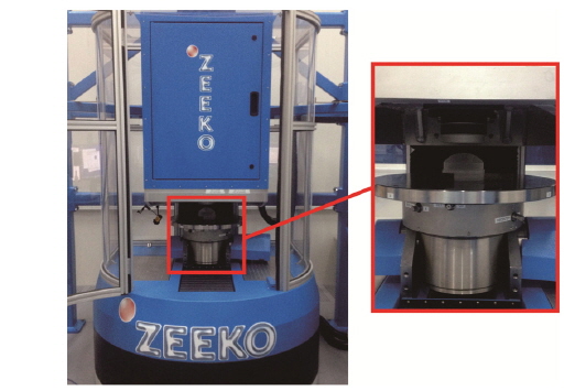
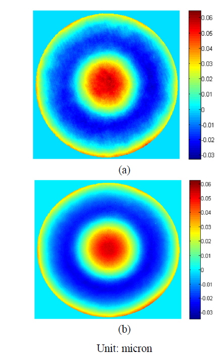
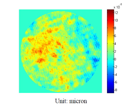
In this section, we test a convex spherical surface (caliber of 100 mm and radius of 76.56 mm) using a sub-aperture stitching interferometer (a Fizeau interferometer whose working wavelength is 632.8 nm) with a reference surface whose F-number is 1.5. A real system including a real sample is shown in Fig. 2. The layout of the sub-apertures is shown in Fig. 3. The measurement results using our algorithm are shown in Fig. 4(a). Comparing with the measurement results obtained using a full-aperture interferometer (shown in Fig. 4(b)), the root mean squared error was 0.003014
We propose a fast algorithm for sub-aperture stitching to quickly compensate for piston, tilt, and defocus errors. We prove that our algorithm runs more than two times faster than the current algorithm. Although the simulation results demonstrate that the accuracy of the new algorithm is lower than that of the current algorithm in all 20 simulations, the new algorithm is sufficiently accurate for generally use. Using an experimental measurement, we verified the validity of the new algorithm and demonstrated successful sub-aperture stitching.