Optical coherence tomography (OCT) is a noninvasive in vivo imaging technique that can provide cross-sectional and three-dimensional volumetric images with high resolution [1, 2]. Following the first demonstration of an OCT image of a human retina, OCT has been applied in various medical fields, including dermatology, cardiology, and bronchology. In addition, there have been significant efforts to realize higher axial resolution, sensitivity, and acquisition speed. Lately Fourier-domain OCT based on either a wavelengths-wept laser (SS-OCT) or a spectrometer (SD-OCT) has become widely used, because of its higher sensitivity and acquisition speed compared to conventional time-domain OCT [3-5].
Ultrahigh axial resolution OCT (UHR-OCT), approaching 3 μm or less in tissue, makes it is possible to obtain images close to the level afforded by histology [6-8]. The axial resolution of OCT depends on the light source’s center wavelength, full width at half maximum (FWHM), spectrum shape, and so on. A broadband light source is often desirable for ultrahigh axial resolution in OCT because this resolution is inversely proportional to the FWHM of the light source [6-11]. Drexler et al. first introduced UHR-OCT using an ultrashort-pulse (< 10 fs) Ti:sapphire laser with a FHWM of 260 nm at 800 nm, and obtained an OCT image of an African frog tadpole with 1-μm axial resolution[6]. Hartl et al.[8] and Leitgeb et al.[9] demonstrated UHR-OCT with a femtosecond-pulse laser coupled with a long optical fiber to generate a supercontinuum. In addition, a superluminescence diode (SLD) combined with several SLD modules was introduced by Ko et al. [10] and Zhu et al [11].
In SD-OCT, a spectral interferogram with a response function linear in the wavenumber (k) must be acquired prior to inverse fast Fourier transforms (FFT). The spectrum of light dispersed by the grating in a conventional spectrometer, which consists of a diffractive grating, lens, and line-scan camera, presents a nonlinear function of the wavenumber (k = 2π /λ). Therefore, a spectral interferogram with a nonlinear function should be rescaled into the k-domain to achieve equal sampling space prior to FFT. Hu and Rollins first introduced a linear-k spectrometer, in which they placed a dispersive prism to remove the rescaling process from the λ-domain into the k-domain at 1310 nm [12]. They used a customized isosceles prism of BK7 material. In the linear-k spectrometer, the only optical parameter considered was the isosceles angle of the prism; the tilt angle between grating and prism was dependent on the isosceles angle of the prism. In this paper, OCT images of a six-layer tape phantom and a human fingernail without a resampling process were successfully demonstrated. Gelikonove et al. simulated the spectrum using a BK7 prism and a prism of non-dispersive material at 1300 nm [13, 14], and found that the contributions to spectrum linearization came mostly from the geometric factors, i.e. the prism angle and the tilt angle between grating and prism, rather than from the prism material's dispersive properties, when they fixed the pitch of the grating and the detected spectrum range. Watanabe and Itagaki optimized the prism material and the tilt angle between grating and prism at 840 nm after they fixed the prism angle, pitch of the grating, and detected spectrum range [15]. They suggested that an F2 equilateral prism was suitable when wavenumbers between 7 µm-1 and 8 μm-1 were detected. In addition, the cross-sectional OCT image of a human fingerprint was presented, with theoretical axial resolution of 6.4 μm in air within an imaging depth range of 3.3 mm. Hagen and Tkaczyk designed compound prisms, such as doublet and triplet prisms, for a linear-k spectrometer [16]. Although the compound prism was intricate, it was designed for use with thermal sources or wideband SLDs.
In this paper, we demonstrate UHR SD-OCT based on a linear-k spectrometer. We simulated optical parameters for prism angle, prism material, pitch of the grating, lens focal length, and imaging depth range of SD-OCT (or spectrum range) before construction of the linear-k spectrometer for UHR SD-OCT. When an F2 equilateral prism, a transmission grating of 1200 grooves, and a lens with focal length of 88 mm were used with a tilt angle of 26.07° between grating and prism, an imaging depth range of 2.1 mm could be achieved. In that case the axial resolution was measured as 3.8 μm in air, corresponding to 2.8 μm in tissue (n = 1.35).
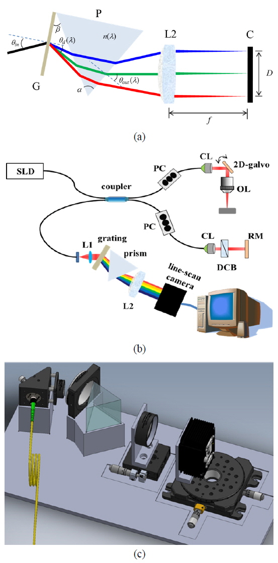
We used used an SLD (BLM2-D-840-B-I-10; Superlum, Ireland) with a FWHM (Δλ) of 100 nm at the center wavelength (λc) of 849 nm, which corresponds to a theoretical axial resolution of 3.2 μm in air, and with an optical power of 10 mW. Figure 1(a) shows a schematic of a linear-k spectrometer. Before construction of our spectrometer, we calculated and simulated several parameters such as prism material, optimal angle between grating and prism, and focal length of the lens by using MATLAB (MathWorks, Natick, MA, USA). When the incident angle is the blaze angle, θin = sin-1(pλc/2), the diffraction angle of light is determined by the diffraction grating equation as following:
where p and M are the groove density of the grating and the total pixel number of the camera respectively. The final output angle, θout(λm), in the prism is [15]:
where α and β are a prism angle and a rotational angle between the grating and the prism respectively, and n(λ) is the refractive index of the prism material. As shown in Fig. 1(a), the spot length (D) of spectrally resolved and focused light depends on the output angle from the prism, the focal length (fL) of the lens:
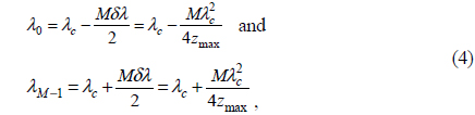
where N is the physical size of each pixel of the camera. λ0 and λM-1, which are the wavelengths of focused light in the first pixel and the last (Mth) pixel of the camera, can be determined by:
where δλ and zmax are the spectral resolution of the spectrometer and the imaging depth range of SD-OCT respectively.
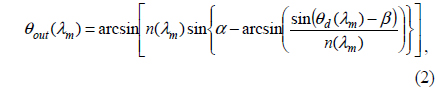
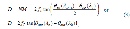
Figure 1(b) shows a schematic diagram of our UHR SD-OCT system. Light from the SLD was incident on a broadband 2×2 optical coupler with 50:50 ratio (Gould Fiber Optics, Millersville, MD, USA) and was split into the reference and sample arms. In the sample arm, the collimated light was incident upon samples via an OCT scan lens (LSM04-BB; Thorlabs Inc., Newton, NJ, USA) with an optical power of approximately 3.5 mW, forming a focal spot with 1/e2 diameter of 24 µm and a 1.15 mm depth of focus. A 2-D galvanometer (GVSM002; Thorlabs Inc., Newton, NJ, USA) was controlled by two analog output channels of a data acquisition board (PCI-6259; National Instruments Corp., Austin, TX, USA). Light reflected from the reference and sample arms was recombined and directed into the linear-k spectrometer. The line-scan camera in the spectrometer had total pixel number of 4096 and a maximum line rate of 70 klines/s (spL4096-70km, Basler, Germany) when all 4096 pixels and single-line acquisition mode were set. However, to increase line rate, we used just 2048 pixels of the camera. When the starting pixel and region of interest (ROI) in the camera were the 1025th pixel and 2048 pixels respectively, the minimum line period of 7.8 µs could be realized, corresponding to a maximum line rate of approximately 128 klines/s. The camera contained two rows of 4096 pixels, so it was operated in “vertical binning acquisition mode” because of the short exposure time of 6.5 μs. When vertical binning mode is used, the same effect is realized as if using a single line sensor of pixel size 10 μm (width) × 20 μm (height). Therefore, we could get increased response efficiency in a short exposure time. In the linear-k spectrometer it was difficult to set the exact incident angle of the grating, tilt angle between grating and dispersive prism, and position of the lens and the camera according to the calculated values. Therefore, we made several mounts according to the drawings shown in Fig. 3(c), based on calculated parameter values.
Spectral data from the camera were digitized by a frame grabber (PCIe-1433, National Instruments Corp., Austin, TX, USA) with a resolution of 12 bits. Acquired spectral data were processed by a personal computer with a quad-core CPU (Intel Core i7-3370; Intel, Santa Clara, CA, USA) and a graphics card (WinFast GTX 680; Leadteck Research Inc., New Taipei City, Taiwan) based on a graphics processing unit (GPU) of the GeForce series (NVIDIA Corp., Santa Clara, CA, USA), which had 1536 stream processors at both a base clock of 1006 MHz and a boost clock of 1058 MHz, and memory of 4 Gbytes at a memory clock of 6008 MHz [15, 17]. To accelerate numerical calculations and display real-time 2-D images, we developed software using Microsoft Visual C++ and NVIDIA’s compute unified device architecture (CUDA) technology.
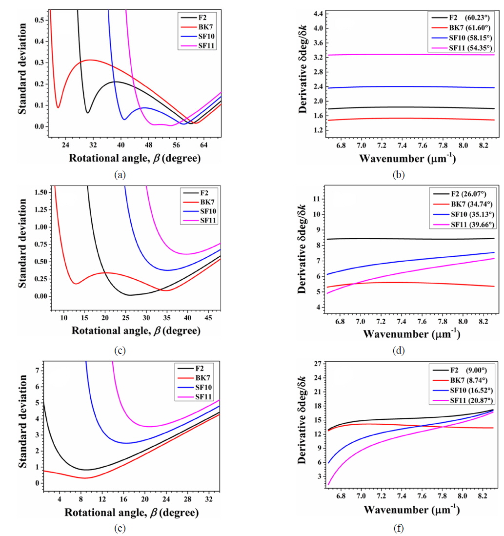
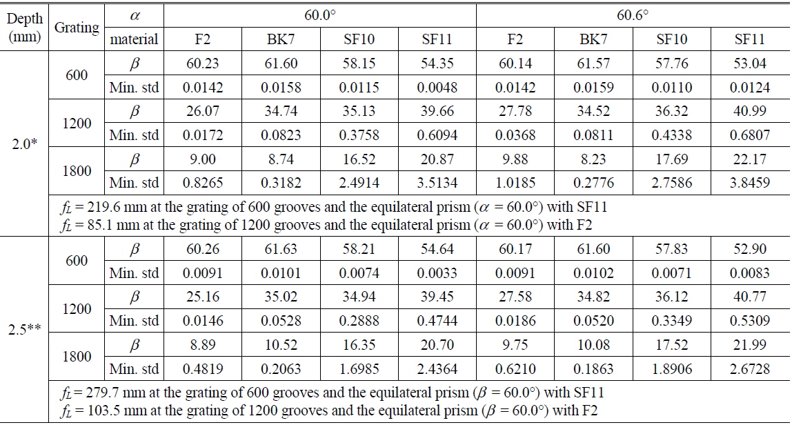
Preferentially, we should choose the imaging depth range of UHR SD-OCT to be 2.0 mm and 2.5 mm, to obtain ultrahigh axial resolution and slow decay of sensitivity (roll-off). The total pixel number of the camera was set to be 2048 pixels, and the physical pixel size in the sensor of the camera was 10 µm (width) × 10 μm (height). Then we calculated β and fL when the pitch of the grating was 600, 1200, and 1800 grooves and the material of the equilateral prism (α = 60.0°) or the isosceles Brewster prism (α = 60.6°) was F2, BK7, SF10, and SF11. We chose these parameters for grating and prism because those components could be easily purchased. The refractive index equation of each material was obtained from Ref. [18]. Figure 2 shows the calculated results for the optimal rotational angle, β, between grating and prism for gratings with 600 grooves, 1200 grooves and 1800 grooves, when the imaging depth range of UHR SD-OCT was 2.0 mm and the prism angle α was 60.0°. The incident angle could be set to approximately 30.7° to match the blaze angle. From Eq. (4), the spectrum from 757.52 nm to 942.48 nm should be detected by a spectrometer with wavenumber resolution (δk) of 7.952 × 10⁻⁴ μm-1 to obtain OCT images with the depth range of 2.0 mm. The optimal angle α and the material of the prism were estimated by minimum standard deviation of derivatives, δdeg/δk, from Figs. 2(a), (c), and (e), according to the number of grating grooves. When the F2 prism was rotated through 26.07° with a grating of 1200 grooves, wavenumber linearity of the spectrometer was sufficient, as shown in Fig. 2(d). In Fig. 2(e), we could find the rotational angle with minimum standard deviation at 1800 grooves, but the function of the wavenumber still presented nonlinearity, as shown in Fig. 2(f).
Finally, from Eq. (3) we could estimate the focal length of the lens to be approximately 85.1 mm. We repeated the calculation while changing the imaging depth range, grating groove count, and prism angle. Table 1 shows the results of the calculations, with optimal material and rotation angle listed in red letters. As shown in Table 1, for a grating with 600 grooves the equilateral and isosceles Brewster prisms of all materials were suitable, because the standard deviation of the derivative (δdeg/δk) for every prism was low (< 0.02). In other words, the linearity of the linear-k spectrometer with a 600-groove grating at 850 nm depended only on the tilt angle between grating and prism, as shown in Fig. 2(b). Additionally, the wavenumber linearity for a grating with 600 grooves was better than for a grating with 1200 grooves. However, if a grating with 600 grooves were used, a lens with a long focal length over 200 mm would be needed. A lens with long focal length comes with the attendant problem that the collimated light incident upon the grating should have a large diameter, over 25 mm, because the pixel size of the camera is small (10 μm × 10 μm). To prepare a large collimated beam over 25 mm in diameter with a broadband light source is difficult and requires a collimation lens with a long focal length. In case of the 1200-groove grating, we found that the tilt angle between grating and prism was slightly different, according to the spectrum range or the imaging depth range of SD-OCT, as shown in Table 1.
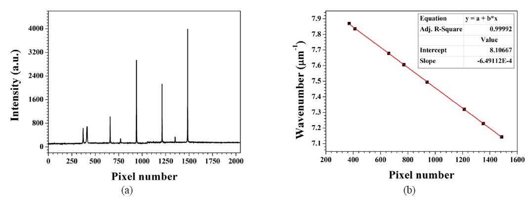
To achieve an imaging depth range of 2.0 mm necessitates a lens with focal length of 85.1 mm, as shown in Table 1. In this study we used achromatic doublet lenses with focal lengths of 750 and 100 mm; the combination of these lenses could yield a focal length of 88.2 mm. Therefore, we could measure the imaging depth range as approximately 2.1 mm. We evaluated the linear-k spectrometer by using a fiber Bragg grating (FBG) array (O/E Land Inc., Lasalle, QC, Canada) at eight different wavelengths [19]. Each FBG had a narrow spectral bandwidth of 0.048 nm and reflectivity of 70-95%. Table 2 shows a look-up table for the wavelength and wavenumber of the FBG array. We blocked reflected light from the reference arm and disconnected the fiber of the optical coupler in the sample arm from the collimation lens, and then the fiber of the optical coupler was connected to the FBG array. The spectrum of reflected light from the FBG array was detected by the linear-k spectrometer, as shown in Fig. 3(a). Spectrum peaks corresponded to each wavenumber of the FBGs in Table 2. When linear fitting analysis of pixel numbers versus wavenumber at spectrum peaks was performed, an adjusted R-squared value of the fitting function of 0.99992 was obtained, as shown in Fig. 3(b). Therefore, we could conclude that our linear-k spectrometer had good linearity of detected wavenumber according to camera pixel number.
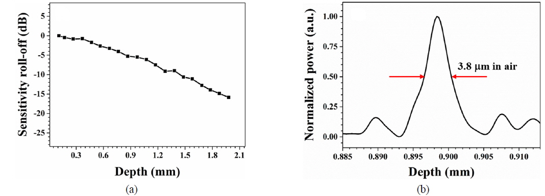
We used a -34 dB partially reflecting mirror as a sample to evaluate the system’s performance, including its sensitivity, sensitivity roll-off, and axial resolution. The sensitivity of our system, determined by adding the sample attenuation constant, was approximately 91 dB at near-zero depth, and a decrease of 10 dB was observed at approximately 1.5 mm, as shown in Fig. 4(a). The attenuated light with -30 dB in the reference arm was also used. Using a 10:90 optical coupler and an optical circulator, the sensitivity could reach up to approximately 94 dB. Figure 4(b) shows the point-spread function of the axial resolution when the mirror sample was positioned at a depth of approximately 0.9 mm. The measured axial resolution was 3.8 μm in air, corresponding to 2.8 μm in tissue (n = 1.35).
To obtain a real-time cross-sectional OCT image, we used the multithreading technique of the CPU and parallel calculation technique of the GPU. First, we acquired and saved spectral interference signals in the memory by using the first thread of the CPU. Acquired interference signals were transferred to the memory of GPU using the second thread of the CPU, and the second thread also asked the GPU to calculate averaging, FFT, and log scaling. When the calculation was completed, the second thread transferred the calculated data from the memory of the GPU to the RAM. The third thread of the CPU was used to display OCT images, and to save BMP files and raw data. In the GPU, spectral interference signals were averaged in the lateral direction, to evaluate the level of the DC signal by averaging the whole spectrum. We subtracted the DC level from each spectral interference signal and performed FFT processing with each spectral interference signal without the DC component. Finally, a logarithmic scaling process was carried out to obtain an OCT image. Numerical k-domain resampling before the Fourier transform was avoided by using the linear-k spectrometer, so the calculation time was reduced. Therefore, we could obtain OCT images with 800 lines/frame at 128.2 fps, which was the theoretical full frame rate, when the probe beam was scanned using a sawtooth waveform with a duty cycle of 80% to reduce mechanical vibrations.
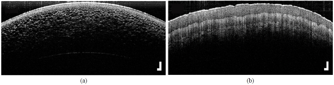
Figure 5 shows OCT images of a cherry tomato and human finger skin with 1024 × 800 pixels, corresponding to a physical size of 2.1 mm (deep) × 9.4 mm (lateral). In Fig. 5(a), membrane layers of small cells in the cherry tomato are clearly visible. In addition, we can see fine structures in the deep region of the finger skin in Fig. 5(b).
In this study we demonstrate UHR SD-OCT based on a linear-k spectrometer. In constructing the linear-k spectrometer, we used simulation results to guide the selection of optical components. According to simulations, a 1200-groove transmission grating, an F2 equilateral prism, and a lens with a focal length of 85.1 mm were suitable for a linear-k spectrometer for UHR SD-OCT with an imaging depth range of 2.0 mm. When we used achromatic doublet lenses (f = 750 mm and 100 mm) in the spectrometer for a focal length of 88.2 mm, we could measure the imaging depth range to be approximately 2.1 mm in air. In that case the measured axial resolution was 3.8 μm in air, corresponding to 2.8 μ m in tissue (n = 1.35). The sensitivity was -91 dB with -10 dB roll-off at a depth of 1.5 mm. Acquisition speed of approximately 128 klines/s could be achieved using half of the total pixels of a camera with 4096 pixels and 70 klines/s. We could obtain OCT images with 800 lines/frame at 128.2 fps (sawtooth scanning, 80% duty cycle) by using multithread processing of the CPU and parallel-calculation processing of the GPU. Finally, we obtained sample OCT images of a cherry tomato and human finger skin.