Analysis of optical devices such as waveguides and directional couplers is essential to be able to predict their characteristics, and involves solving the Helmholtz equation. Meanwhile, analysis of tunneling phenomena is necessary in various problems of particle physics, as well as in certain quantum devices, which requires solving the Schrӧdinger equation. Despite their apparent differences, the two problems are quite closely related from a theoretical standpoint, because the two equations are nearly identical in form. Whatever the structure, one must decide whether to employ a numerical method, or to rely on a mathematical approach for analysis. As to numerical methods for solving the wave equation, one may choose one of the well-known simulation techniques such as FEM (finite element method), BPM (beam propagation method), the TM (transfer matrix) method, and so on, depending on the given application. Numerical methods provide very accurate results, but not necessarily physical insight. On the other hand, mathematical approaches provide such insight, allowing closed-form solutions, but are limited in their use since exact solutions are available only for specific cases such as linear, exponential, and inverse hyperbolic cosine index profiles.
Thus, for a majority of graded structures, many have resorted to approximate mathematical methods. One of the most widely used methods for handling this class of problems is the WKB (Wentzel-Kramers-Brillouin) method. It is well known that results of this method tend to deviate from the exact solution on the whole since trial solutions diverge at the turning points [1]. Despite this deficiency the WKB method has frequently been employed by many researchers [2, 3] owing to the simple mathematical expressions involved, availability of eigenvalue equations in closed forms, and easy estimation of final results. In an effort to circumvent such inherent deficiency of the WKB method, Langer [4] proposed a method utilizing the Modified Airy functions (MAF), which was later applied to the analysis of optical waveguides and also to tunneling problems in connection with potential barriers by Ghatak et al. [5, 6]. More recently, Kim et al. applied the MAF method to a variety of optical waveguides [7, 8] and tunneling problems [9, 10] by employing MAFs in constructing the trial solution across the entire structure, demonstrating the method’s accuracy. Despite these recent advances, however, researchers have failed to clearly point out that the method does not yield satisfactory results in cases where particle energy is comparable to the barrier peak, for some classes of potential barrier profiles, and have not provided a rational explanation for such behavior. This work aims to address these shortcomings.
This paper is comprised as follows. First, the basics of the MAF method are addressed, with an optical waveguide as the platform for discussion. A trial solution is presented for each distinct region, followed by the corresponding ‘connection formula’. Then actual application of the MAF technique to the analysis of graded-index waveguides is presented. Using the MAF trial solutions, a closed-form expression of the eigenvalue equation is derived for graded-waveguides. The eigenvalue equation is then solved for several graded-index profiles, to yield the dispersion curves. The results are shown to be in very good agreement with exact numerical results obtained using the FEM.
The second part comprises the analysis of the tunneling problem. Based on the same MAF trial solutions postulated in the waveguide case, tunneling probability is derived in matrix form and evaluated for a number of graded potential barriers. The results are compared with exact numerical solutions obtained using the TM method, whose accuracy has already been verified in numerous studies [11, 12]. It turns out that MAF method fails for profiles with a smooth peak and that the WKB method does not work as well for profiles with an abrupt truncation or change.
Possible causes for the discrepancy in accuracy of the results for waveguide and tunneling problems upon application of the same MAF method are investigated in a systematic manner. This evaluation has not been previously addressed, to our knowledge. In the process, the corresponding results of the conventional WKB method and the FEM or TM method – the latter two providing exact numerical solutions – are also presented for comparison.
II. MAF TRIAL SOLUTIONS AND CONNECTION FORMULAE
In this section, a brief overview of the MAF method is presented. Although the discussion is conducted for optical waveguides, the formulation and basic concepts apply equally to the potential-barrier problem.
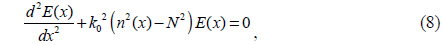
Let us start with the one-dimensional wave equation for optical waveguides:

where

In (2),
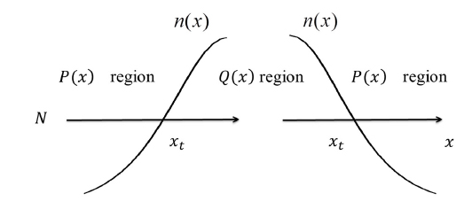
In Fig. 1 a diagram of Γ(
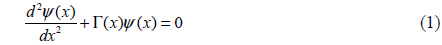
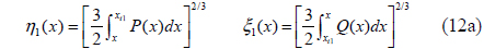
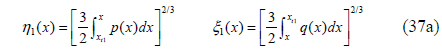
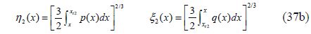
Let us at this point define the following auxiliary functions for subsequent discussions.

where

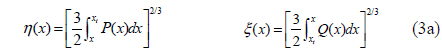
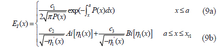
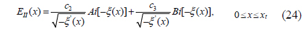
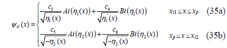
The MAF trial solutions to (1) are given by a combination of the modified Airy functions as follows:

where
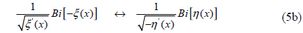
Note that


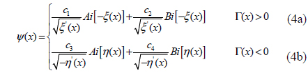
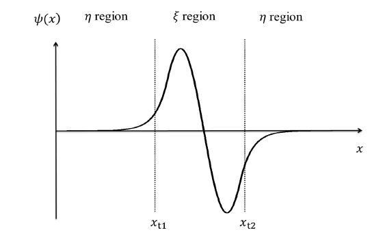
The connection feature of the trial solutions presented in (4) can be seen more clearly through the behavior of a typical wave function, shown in Fig. 2 below.
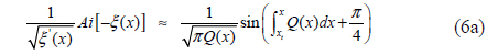
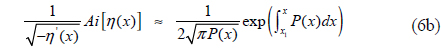
The MAF trial solutions of (4) take on the following asymptotic forms away from the turning point


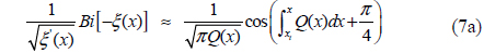
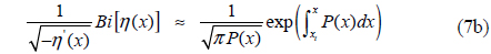
The expressions on the right-hand side of (6) and (7) constitute the well-known WKB connection formula, by which (6a) and (7a) are correspondingly transformed into (6b) and (7b), respectively.
III. APPLICATIONS OF THE MAF METHOD TO OPTICAL WAVEGUIDES
3.1.1. Derivation of Eigenvalue Equation
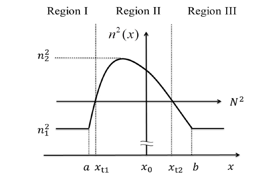
Consider a planar waveguide with an arbitrary graded-index profile, as shown in Fig. 3.
The one-dimensional Helmholtz equation is

where the mode index

where

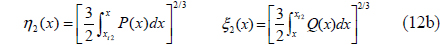

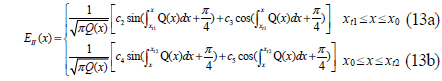
Away from both turning points, the expressions in (10) can be replaced by a linear combination of the sinusoidal functions of (6) and (7), as shown below.

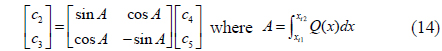
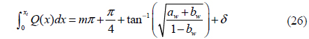
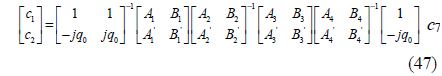
One way to obtain the eigenvalue equation is simply to equate (13a) and (13b). Simple algebraic manipulations lead to the following result.

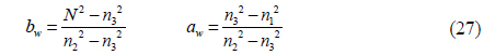
Another way is to impose boundary conditions requiring that the field and its derivative be continuous at
Both approaches lead to the same eigenvalue equation.

In the expression above,

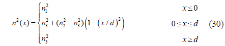
Expressions for


where
For a symmetric profile,
3.1.2. Simulation
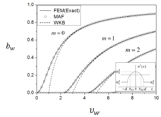
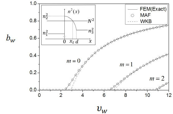
To validate the eigenvalue equation of (15), the following parabolic index profile (shown in the inset of Fig. 4) will be assumed.

To facilitate computation, the normalized frequency

(15) can then be cast in the following form, below which the corresponding WKB eigenvalue equation is also presented, for reference.


The normalized dispersion curves
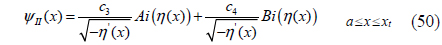
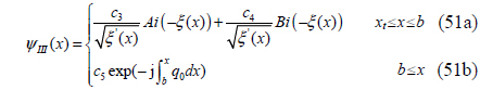
3.2. Truncated Graded-Index Waveguides
3.2.1. Derivation of Eigenvalue Equation
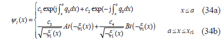
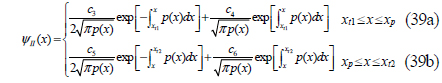
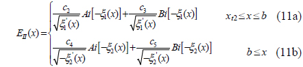
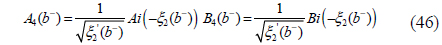
Consider a truncated graded-index profile, as shown in the inset of Fig. 5. Notice that the left turning point now coincides with the location of the index discontinuity. MAF trial solutions appropriate for this structure can be written as follows.

where the definitions of
By applying a procedure similar to that of the previous section, the eigenvalue equation can be obtained as follows.

where

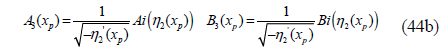
While the
where
3.2.2. Simulation
The truncated parabolic index profile of Fig. 5 is described as

For this truncated profile, the eigenvalue equation of (26) can be cast in the following form. The WKB eigenvalue equation is also presented, for reference.

Calculation results based on the eigenvalue equation of (31) are displayed in Fig. 5 along with the corresponding WKB and FEM results. As was the case for the symmetric parabolic index profile (see Fig. 4), the MAF results show excellent agreement with the exact FEM results, while the WKB curves show minor deviations near the cutoff regions.
Based on this and the previous result, it may be concluded that the MAF technique provides a rather robust and highly accurate method for analysis of a wide range of graded-index optical waveguides.
IV. APPLICATIONS OF THE MAF METHOD TO TUNNELING PROBLEMS
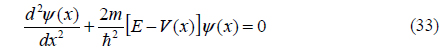
The MAF-based approach will now be applied to a set of barrier profiles, to test its feasibility in tunneling analysis. The one-dimensional Schrӧdinger equation takes the form
Hereafter, we will work in atomic units where
4.1. Graded Potential Barriers
4.1.1. Derivation of Tunneling Probability
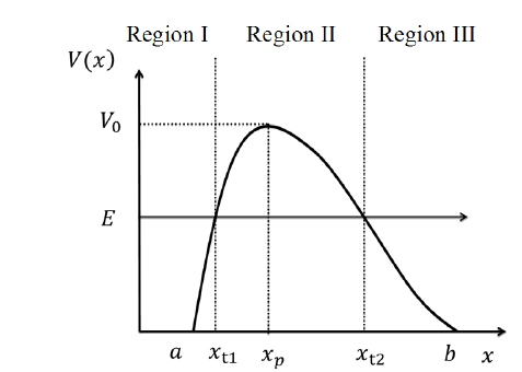
Consider a potential barrier as shown in Fig. 6, with particle energy

where


Suppose the expressions of (35) are replaced by the following asymptotic forms (see Appendix A) much like in the earlier waveguide section but with different forms here.

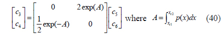
Either by equating these two equations or by imposing the boundary conditions at a point between the two turning points, the following relation may be obtained.

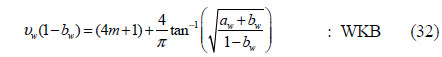
At this point, it must be noted that the computation results based on (40) were nearly identical to those obtained from the WKB analysis. This is in clear contrast to the case of the optical waveguide, where use of asymptotic forms of the MAF trial solutions led to very accurate results that were distinctly different from the WKB results.
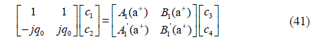
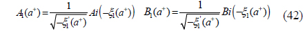
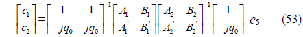
We shall now revert to the trial solutions of (34) to (36) as they are, and impose the boundary conditions at

where
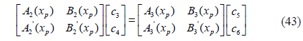
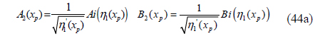
Next, boundary condition matching at

where

Finally, application of the boundary conditions at
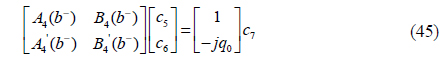
where
Equations (41), (43), and (45) can be combined to yield the following overall matrix equation relating
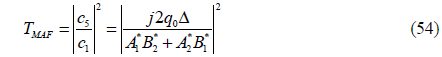
It follows from (47) that the tunneling probability is given by the expression below.

Detailed descriptions of the terms ∆1, ∆2,
Derivation of the tunneling probability using the WKB method for a graded potential barrier is presented in Appendix B-1.
4.1.2. Simulation
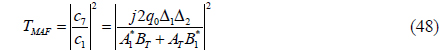
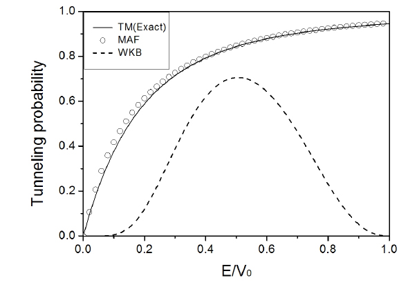
Case 1: Symmetric exponential potential barrier
To verify the validity of the MAF formulation for graded potential barriers, a symmetric exponential profile (shown in the inset of Fig. 7) was selected as the first test case. The calculated results based on (48) are displayed in the figure, along with the results obtained by the exact transfer matrix (TM) method. The WKB results are also included, for reference.
Figure 7 clearly shows that the MAF method leads to solutions with very high accuracy over the entire region of
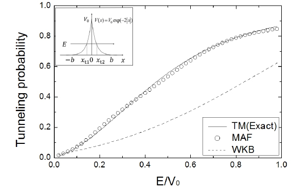
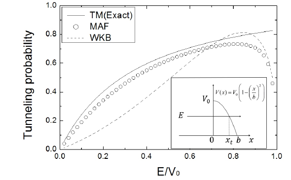
Case 2: Parabolic potential barrier
A parabolic potential barrier is taken as the second example, and is shown in the inset of Fig. 8.
Calculated results for this profile are illustrated in Fig. 8. The WKB results show behavior similar to that in Fig. 7. However, the MAF results show tunneling probabilities much lower than the true values across the entire range, contrary to expectation; part of this tendency can in fact be observed in the previous reports of [6, 11] upon careful examination. Even more disturbing, the calculation results fall to zero as
4.2. Truncated Potential Barriers
4.2.1. Derivation of Tunneling Probability
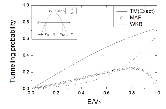
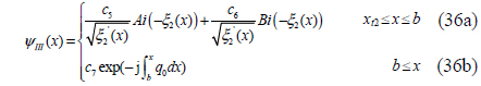
Consider a truncated graded potential barrier, as shown in Fig. 9.
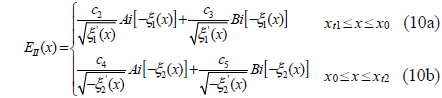
For the truncated graded barrier in Fig. 9, the trial solutions may be taken to be

where
By applying the boundary conditions at
It follows that the tunneling probability is then given by
Detailed descriptions of the terms ∆,
4.2.2. Simulation
Here the same two potential profiles analyzed in the previous section shall be examined, but with the left half of each profile removed.
Case 1: Truncated exponential potential barrier
Let us take the truncated exponential potential barrier of the inset of Fig. 10 as the first example.
The calculated results based on (54) are displayed in Fig. 10, which shows excellent agreement between the MAF results and the exact TM results. It is seen that the WKB results, on the other hand, fail: As
Case 2: Truncated parabolic potential barrier
A truncated parabolic potential barrier, shown in the inset of Fig. 11, is taken as the second example.
Simulation results are illustrated in Fig. 11. The results are interesting in that both the MAF and the WKB curves deviate significantly from the exact solution, and fall to 0 as
The plausibility of applying the MAF method to the analysis of graded optical waveguides and potential barriers was reviewed in this paper, with the conventional WKB method serving as a basis for comparison. Application of the MAF technique to the waveguide problem led to satisfactory results for both symmetric and truncated graded-index distributions, in that it was possible to derive a simple closed-form eigenvalue equation, and the calculated results were very accurate. When the same MAF approach was applied to the problem of tunneling probability in the presence of a graded potential barrier, however, the results were mixed, which was contrary to our initial expectation. The MAF method turns out to be inadequate in any case with
The discrepancy between the end results from the MAF analysis for the two classes of problems, graded-index optical waveguide and graded potential barrier, is believed to stem from the different respective natures of the two problems. In the waveguide problem only discrete eigenvalues are allowed, and any mode index
It may thus be concluded that the MAF method is not appropriate for analysis of tunneling problems in which graded potential barriers with the condition of