Moiré interferometry is the most commonly used method for examining long focal lengths and is based on the Talbot effect and Moiré fringe analysis [1-3]. When a plane wave is incident upon a periodic transmission grating, a self-image of the grating is formed at regular distances from the grating, the so-called Talbot distance and its multiples, and a similar phenomenon occurs when a grating is placed in a converging or diverging beam. In this case the self-image of the grating becomes (de)magnified and the magnification, which depends on the convergence of the beam and on the distance away from the grating, is the key aspect for determining the focal length of the lens. To determine the magnification, the 2^nd grating is normally placed at the (de)magnified image of the 1^st grating to form a superimposed pattern of the two gratings, the so-called Moiré fringe. The 2^nd grating is normally rotated by a small angle with respect to the 1^st grating and the angle between the gratings affects the Moiré fringe overall. Therefore, precise information on the angle between the gratings is as important as analyzing the fringe accurately.

This paper presents a simple way of determining the magnification by analyzing the (de)magnified Talbot image directly. Neither Moiré fringe analysis nor the information on the 2^nd grating is required.

To demonstrate the validity of the method, two aspects need to be considered: the accuracy of the determination and an accurate method to determine the (de)magnification. To address the accuracy, this paper presents a set of numerically-simulated Talbot images by propagating a converging beam numerically (using a two-step transfer function approach to calculate the Fresnel diffraction integral) through a binary grating and to a detector. A long-focal-length system to be tested with the Talbot images formed by a grating, which is relatively small in size, can be represented with a high F/#, which guarantees that the numerical simulation is correct, and the set of specifications used for the simulation can be regarded as references or true values. Therefore, the difference between the analyzed values and true values can represent the accuracy of the method, which is described below.

One of best analyzing methods for the periodic images is to employ a Fourier transform, and a fast Fourier transform (FFT) is normally used for the frequency spectrum of the image because of the fast execution time. One drawback of the FFT is that the frequency spectrum consists of a finite number of values with a finite frequency interval given by the side length of the fringe image due to sampling the fringe. The original Fourier transforms (OFT) were employed to access the frequency spectrum beyond the limitation. The process was also iterated a number of times for better accuracy.

A set of numerically simulated Talbot images was used to demonstrate the validity of the proposed method.

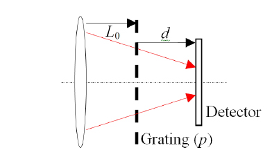
Figure 1 shows a schematic diagram of the setup in which a positive lens causes a beam to converge as it propagates through a binary grating with period of p and to a detector. The grating is located at an arbitrary distance, L₀, from the lens and the detector is located at the distance, d, from the grating, where a (de)magnified image of the 1^st grating is measured.

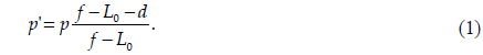
The (de)magnified period of the 1^st grating, p′, at the detector can be calculated using similar triangle properties with the help of Fig. 1, as follows:

If L₀ is measured from the back surface (the principal plane) of the lens, f will be the back (effective) focal length. Here the distance d is called the Talbot distance if the beam is collimated. For converging or diverging beams, the Talbot distance would be modified slightly [1]. It is important to have a sharp (de)magnified-image to form an optimal image with an accurate measurement of the distance between the grating and detector for a focal length determination. With the measured (de)magnification, p′/p, the focal length of the lens can be expressed as

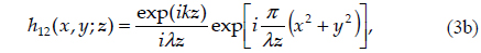
The simulation was composed of two elements: numerical beam propagation and an implementation of a binary grating with respect to an array representing the optical field in the simulation. An aperture was not needed in the actual experiments, but a circular pupil in contact with the test lens was used for the simulation. The beam was then propagated through the grating to generate a Talbot image. Both the propagation from the pupil to the grating and that from the grating to the detector were calculated using the Fresnel diffraction integral with a two-step transfer function approach, given by [4]

where the impulse response is given by

where z is the propagation distance and k(=2π/λ) is the wave-number of the beam. The optical field u(x,y) is represented by an array of complex numbers and the symbol * in Eq. (3a) represents the convolution, which was carried out using the two-step FFT approach for optical field arrays [4]. The same numerical beam propagation was used to simulate the Ronchigrams [5]. To verify the numerical beam propagation, the beam size of a converging circular beam without aberrations as a function of the propagation distance was calculated. With proper sampling of the initial beam to avoid aliasing during the numerical propagation, the linear dependence of the beam size on the propagation distance was confirmed. The numerical simulation was developed as a MATLAB-based program [6].

The grating is treated as an amplitude filter during beam propagation; the grating is also represented by an array of real values, and each element of the array (hereafter, we refer to each element as a pixel) is assigned a value between 0 and 1, where 0(1) corresponds to the case where the beam is blocked (transmitted) completely. The grating was assumed to be aligned vertically, and the first row of the corresponding array was filled with values between 0 and 1 depending on the period of the grating and the pixel size. A fractional value was assigned to the pixels that corresponded to the edges of the grating. The subsequent rows of the array were duplicates of the first row, to represent the vertical binary grating. The grating was assumed to be a binary transmission grating with a square wave profile and a 50% duty cycle.

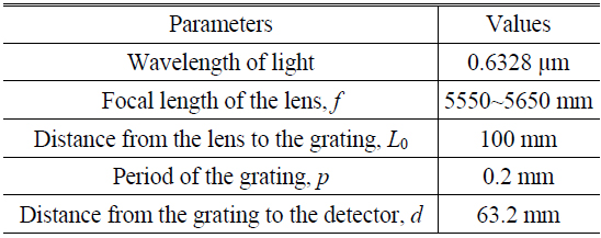
To discuss the period analysis, a set of simulated Talbot images was generated using the simulation system with the specifications listed in Table 1. To avoid aliasing due to insufficient sampling in the simulations, an array of 2048×2048 was used for the numerical beam propagation, and a circle of diameter 2000 pixels (where each pixel has a side of length 0.01 mm) was used to simulate a circular beam with a diameter of 20 mm. The distance from the grating to the detector was set as the first Talbot distance.

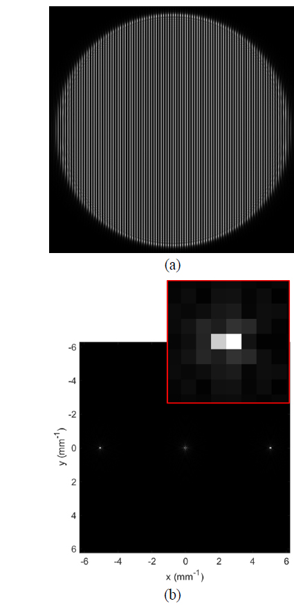
Figure 2(a) shows the simulated Talbot image for the focal length of 5600 mm and Fig. 2(b) presents the spatial frequency spectra calculated by FFT for the simulated image. The frequency spectrum is also an array of size, 2048×2048, due to the array size for the image. Because the important information is located near the origin of the spectrum, Fig. 2(b) only shows a partial array of size of 256×256 near the origin. The frequency spectrum at the origin is the sum of the intensities of all the pixels, and the rest of the spectrum becomes almost zero if the spectrum is normalized to it. Therefore, the spectrum at zero frequency was set to zero, and the rest of the spectrum was normalized to the intensity to fit into an 8-bit grayscale (with 256 grays) with black (white) being the minimum (maximum) intensity. Using the known length of the image (20.48 mm), the spatial frequency interval corresponding to each pixel in the spectrum can be calculated as 0.0488 (= 1/20.48) mm⁻¹, and the (de)magnified period of the image can be calculated from the peak of the frequency spectrum if the spectrum peak is well defined, as shown in Fig. 2(b), where the peak is located at a pixel offset of (104,0) or (−104,0) from the origin. zand the (de)magnified period is 0.1969 mm (=20.48/104), whereas the precise corresponding value is 0.1977 mm, as calculated by Eq. (1). If the coarse (de)magnified period is used to determine the focal length of the lens, Eq. (2) equals 4208 mm, which is 1392 mm away from the true value.

One way to improve FFT analysis is to apply the center-of-mass algorithm to calculate the centroid of the spectrum peak. With the algorithm, the centroid of the 5×5 pixels centered at (104,0) from the origin turns out to be (103.652,0) from the origin, which corresponds to a spatial frequency of 5.0611 mm⁻¹. Therefore, the corresponding focal length becomes 5332 mm, which is better than previous one with a difference of 268 mm.

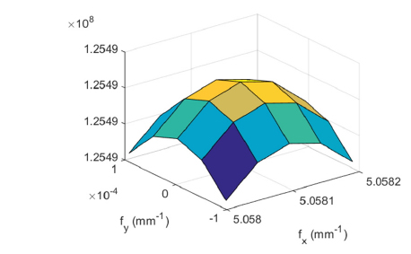
To calculate the centroid of the spectrum peak with much higher accuracy, the alternative to the FFT was considered. The FFT was developed to reduce the execution time by sacrificing the frequency components. Therefore, the original Fourier transform (OFT) was utilized and the exact procedure is as follows: 1) a square region of the spectrum centered on the spectral peak obtained by the FFT is divided into a 5-by-5 grid of frequency components; 2) the spectra for the frequency components are calculated with the OFT; 3) among the 25 spectra, the maximum component is searched for and found; 4) a new square region, which is centered on the new component and has a side length that is half that of the previous region, is subdivided again; and 5) the searching procedure is repeated a number of times. Figure 3 presents the surface plot of the 25 frequency spectra after 9 iterations of the OFT procedure. The symmetrical shape of the surface plot validates the procedure and the top of the surface corresponds to the centroid of the spectrum peak, which is (5.0581, 0) mm⁻¹. The (de)magnified period can be calculated using the centroid of the peak of 0.197703 mm and the determined focal length of 5602.8 mm. The difference is only 2.8 mm

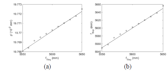
Once the accuracy of the focal length with OFT analysis is achieved, a set of Talbot images is simulated numerically for the system with the specifications listed in Table 1 and the focal length ranging from 5550 mm to 5650 mm, and Fig. 4 shows the (de)magnified periods and the corresponding focal lengths determined with OFT as a function of the focal length, respectively. The standard deviation of the difference in the determined focal lengths is 3.8 mm and the average difference is 3.3 mm, indicating an accuracy of approximately 0.06 %.

This paper presented a method for determining the focal length with Talbot images. Neither the Moiré fringes nor mathematical calibration was used, but applying the original Fourier transform to the (de)magnified Talbot images demonstrated that the true values can be recovered with sufficient accuracy to determine the focal length of the system. The setup is much simpler than the usual setup with Moiré fringes, and the simple apparatus certainly means fewer factors that affect the measurements. The (de)magnification depends on the distances between the elements as well as the image quality. A study of these dependences and further improvements will be the subject of future work.