The Gaussian (or paraxial) image plane (GIP) is the location of the object-like sharp image for aberration-free systems and serves as a fundamental reference of the object for all other geometrical optics characteristics. When the object is distant, the GIP becomes the focal plane, which is one of the cardinal points. The focal length is defined as the distance from the nodal or principal point, another cardinal point, to the focal plane, while the reciprocal of the focal length gives the refracting power of the system. This allows the system to be designed to meet specific requirements [1]. Aberration is also defined as the difference between the wavefront at the exit pupil and the reference sphere with center located at the GIP [1].

To determine the location of the nodal point, the nodal slide technique serves as a standard method [2], and several methods exist for determining the focal length, the Talbot effect approach being one such example [3]. However, it appears that no report exists on the determination of the GIP location, which is the focus of this paper.

For aberration-free systems, rather than displaying a point at the GIP, a slight defocus from the GIP enlarges and blurs the image spot of an axial point object. For actual physical systems, however, the degraded image spot becomes overcast because of the effects of aberrations, mainly primary spherical aberrations, and the image spot itself cannot be distinguished from the defocus and spherical aberrations. In addition, diffraction and interference within the focal region are still unavoidable. According to 3^rd-order aberration theory, the optimal image point can be acquired if the primary spherical aberration is known a priori, which is not the case in typical physical systems. However, we previously measured both spherical and defocus aberrations as a function of the Ronchi ruling locations in the Ronchi test, and the location of the GIP was determined under the assumptions of 3^rd-order aberration theory [4].

In this paper, we extend the usual definition of the transverse magnification (TM) in terms of paraxial ray tracing to the image plane (IP), which is assumed to be displaced from the GIP, and find that TM depends linearly on not only the displacement of the IP from the GIP, but also the location of the small circular aperture stop (AS) placed in front of the system under test. While the former dependence can be understood based on the pinhole effect [5], the latter dependence has not been reported previously. With both dependences, we are able to characterize the location of the GIP as the point at which the slope of the TM variation changes sign. This description is sufficiently deterministic and self-consistent that no other parameters or measurements are needed.

Note that the TM measurements require a set of off-axis point objects, and another aberration, distortion, is inevitable and prevents the TM measurements from being determined properly and accurately in normal circumstances. To overcome this issue, we use our recently developed analysis for distortion [6, 7], which can estimate an average error of 0.09% in the distortion for smartphone cameras over a full range of conjugation [8]. Therefore, a set of experimental data for a thick bi-convex lens system is presented to validate the description.

Paraxial ray tracing, called the y-nu method, is described in most geometrical optics textbooks [1], and is normally used to calculate the location of the GIP for a given object plane by tracing the so-called marginal ray. If a second ray is traced, called the chief or principle ray, a full analysis of Gaussian optics can be completed for the system under test. The transverse magnification (TM) is usually defined as the ratio of the chief ray heights at the object plane and at the GIP. In this paper, however, an IP which is displaced from the GIP is considered and the definition of the TM is extended to the displaced IP (hereafter we use this definition of TM for all cases). Figure 1 shows the paraxial layout for a thick lens imaging optical system with surfaces labeled planes number 1 and 2. The object plane is marked 0 and the IP is 3, while the displacement of the IP from the GIP is denoted by δ₂.

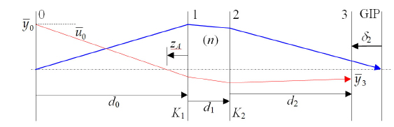
A conventional marginal ray, whose ray height is 0 at the object plane and which is represented in Fig. 1 by a blue arrow, is traced to the GIP. The condition that the ray height must be zero is used to find the distance to the GIP from the 2^nd plane, d_2,GIP, according to

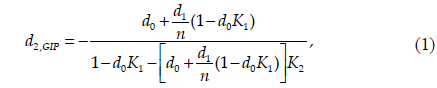
where n indicates the refractive index of the lens; K₁ and K₂ represent the refracting powers of planes 1 and 2, respectively; and d₀, d₁, and d₂ are the distances between the object plane and plane 1, plane 1 and plane 2, and plane 2 and the IP, respectively. The typical sign convention is used [1].

To trace the chief ray, represented by the red arrow in Fig. 1, the AS of the system must be specified. Instead of drawing the AS in Fig. 1, its location is denoted by the variable, z_A (<0 for the configuration shown in Fig. 1), to the left of the first refracting surface of the system. Based on the sign convention, the chief ray angle variable, , can be expressed as

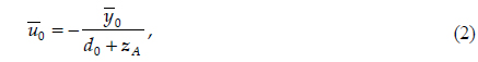
where is the ray height at the object plane. The chief ray height, , at the displaced IP (not the GIP) can be written as

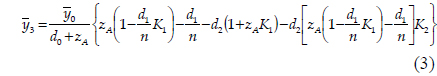
If d₂ = d_2,GIP for the GIP, Eq. (3) becomes the usual simple equation, where

The TM, the ratio of the ray height at the displaced IP to that at the object plane, can be obtained by simply deleting the ray height at the object plane term from Eq. (3), such that

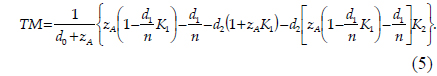
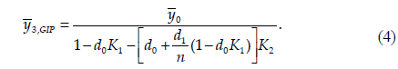
Once again, the TM at the GIP can be obtained if d₂ is substituted into Eq. (1), with

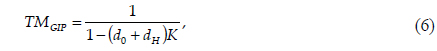
where the denominator has been simplified by the inclusion of the total refracting power of the system, K, and the distance from the 1^st-plane to the object-side principal plane, d_H, which are expressed as

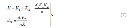
Eq. (6) is equivalent to the thin lens equation, TM_GIP = 1/(1-pK), where K is the refracting power of a thin lens and p is the object distance to the thin lens, which is the sum of d₀ and d_H for the system represented in Fig. 1, by definition [1].

It is worth noting that, in practice, the experimental set to determine the Gaussian image plane of any multi-lens system for an object should treat the system as a whole as a single element, for example, as a thick lens, which is the approach adopted in this paper. The conversion from a multilens system to a single element system can be equivalently achieved without any losses [1]. That is, the two refracting surfaces can be taken to represent the actual first and last refracting surfaces of the multi-lens system. In addition, the surface of the detector that is defined as an IP and a circular aperture located in front of the system (in the experiment that will be described in detail below and as shown in Fig. 1) are the two most important elements to be considered during the experiment.

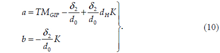
Eq. (6) shows that the TM at the GIP does not depend on anything but the elements described above, as expected. In contrast, when the IP is not on the GIP, the TM is no longer a constant but a function of various parameters, as shown in Eq. (5). In order to determine the relationship between the TM and the AS and IP locations, Eq. (5) must be rearranged. From Eq. (6) and the expression d_2,GIP=d₂−δ₂, Eq. (5) can be rewritten as

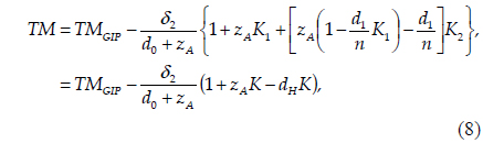
where the minus sign of the second term is due to the fact that the IP is displaced to the left of the GIP, according to the sign convention [1]. Note that no approximations were used to achieve the simplification from Eq. (5) to Eq. (8).

Eq. (8) indicates that the TM depends on the location of the AS, as well as that of the IP. The fact that the TM is linearly proportional to the displacement, δ₂, can be understood as being a pinhole effect [5]. In order to understand the linear relation between the TM and AS location, however, an approximation is needed. If the magnitude of the variable, z_A, is assumed to be much smaller than the distance, d₀, then the variable in the denominator in Eq. (8) can be ignored and the second equation in Eq. (8) can be simplified as a linear function of z_A. Thus,

where the intercept and slope are given by

Ideally, the TM does not depend on the location of the AS when the IP is exactly on the GIP. However, the IP in any physical system cannot be located exactly at the GIP and, therefore, the IP can be considered as being displaced from the GIP by some amount, without the loss of generality. In this paper, this fact is assumed at the outset.

If the location of the AS is varied over a short range and the corresponding TMs are measured, they will vary linearly with distance from surface 1 to the AS, and the slope of the TM variance will be given by the level of displacement of the IP, as shown in the second expression of Eq. (10). If a set of similar measurements is repeated for a set of different IP locations, the slopes will vary accordingly. Eventually, the sign of the slope will change as the IP crosses the GIP. Thus, the GIP location can be determined as that of the IP for which the sign of the slope changes from positive to negative or vice versa.

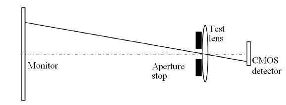
To demonstrate the method described in Sec. 2, the experimental setup shown in Fig. 2 was utilized for a series of measurements to be conducted. We used our previous work on distortion analysis to obtain accurate and precise measurements of the transverse magnification [6, 7]. Briefly, a 15” LCD monitor (pixel pitch = 0.294 × 0.294 mm²) was used as an object plane to display a number of bright pixels in a square grid (55 × 55) as point sources, and a circular AS of diameter 3 mm was placed in front of a bi-convex testing lens (BICX-25.4-23.9-C, CVI Melles Griot, f = 24.8 mm at λ = 546 nm). The pixels of the point sources were turned to maximum intensity (= 255 intensity) and all other pixels were turned off (= 0 intensity). The resultant images were obtained on a monochromatic CMOS detector (Mightex Systems) with a detector pixel pitch of 5.2 × 5.2 μm². Finally, the camera was positioned at the optimal focus location and the gain and exposure time were adjusted so that the peak intensity was under the saturation level.

Each measured image was composed of spots that resemble the pattern of the bright pixels on the monitor, and the spot coordinates in the image were analyzed and processed using a set of fitting procedures, as described in Ref. 6. The tip/tilt angles were minimized and the distortion center was aligned to the optical axis as far as possible. The transverse magnification measurements were then performed.

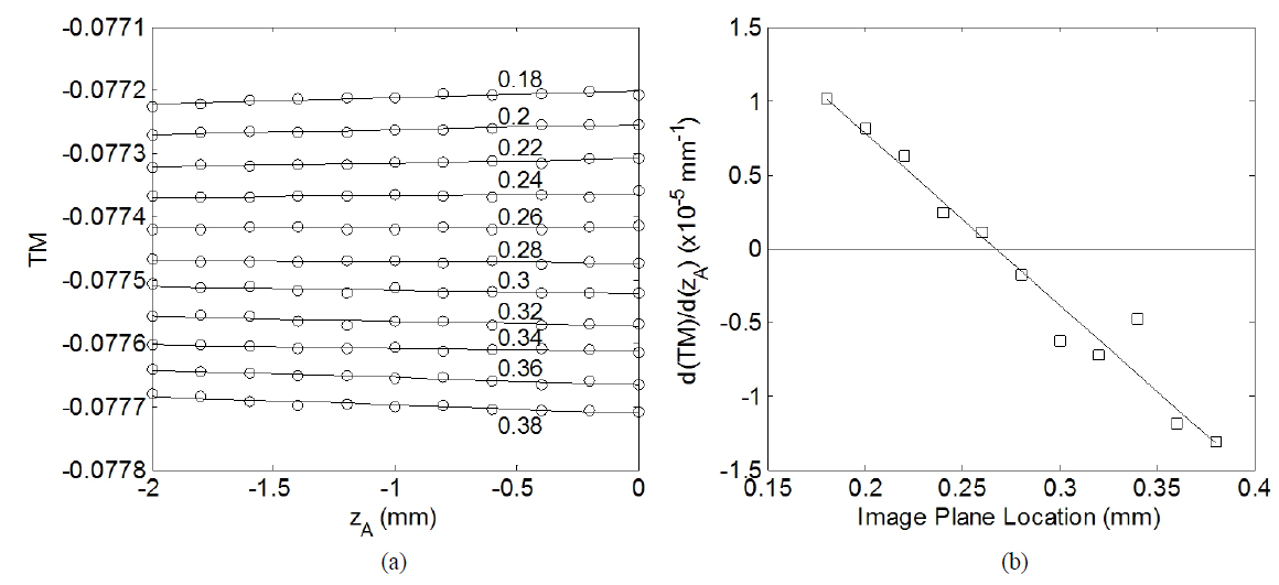
For an IP that was located initially at an arbitrary location near the GIP, the AS was placed at a set of 10 different locations in front of the lens with an increment of 0.2 mm and the corresponding TMs were measured. The AS locations were measured with respect to the front lens vertex with a precision of 0.01 mm. Then, the IP was further displaced from the lens by 0.02 mm and the same set of measurements was repeated. Figure 3(a) shows the measured TMs as a function of the AS for various IP locations whose micrometer readings are given along with the corresponding data. This figure clearly shows that the TM trends conform to expectation based on Eq. (9) and (10): they are increasing for the IP located at 0.18, decreasing at 0.38, and almost constant at 0.28. To quantify these trends, each set of TMs was fit to a linear function and the solid lines were calculated based on the best fit values, as shown in Fig. 3(a).

In order to determine the linear variance of the slopes in response to varying IP location, the best fit slopes, d(TM)/d(z_A), as functions of IP location were plotted, as shown in Fig. 3(b). While the slopes of the TMs for the IPs located between 0.18 mm and 0.26 mm are positive, those between 0.28 mm and 0.38 mm are negative, indicating that the GIP is located between 0.26 mm and 0.28 mm. To calculate the numerical value, another linear function was fit to the set of slopes and IP locations, and the slope and intercept were used to compute the GIP location, yielding a result of 0.27 mm. The solid line in Fig. 3(b), which was calculated using best fit values, clearly demonstrates the linear relationship between the TM and the AS, and also the IP location, as described in Sec. 2.

In this paper, the Gaussian image plane of an optical system for a given object has been redefined as the position at which the slope of the TM variance changes sign. Based on this definition, a method of locating and measuring the GIP has been derived and evaluated. In a practical experiment, a series of transverse magnification measurements for a thick bi-convex lens system with known locations of the IP and a circular aperture was conducted. It was found that the TM varies linearly with the aperture location, as predicted, and that the slope of the variance varies linearly with the IP location. The measurements clearly validate the theory and method described above and confirm that the redefinition of the GIP given in this paper is correct.