The use of renewable energy sources is rapidly developing, and the application of solar energy focusing photovoltaic systems is becoming increasingly popular. The major challenge in photovoltaics is posed by the instability, nonlinearity, and complexity of the current-voltage characteristic equation. In this paper, we propose an intelligent control of a three-phase photovoltaic grid-connected inverter system, which is essential to consider. The behavior of photovoltaic’s in current-voltage and voltage-power is described by complex and nonlinear analytical equations, and depends on various levels of solar intensity and various cell temperatures. The characteristic of photovoltaic’s is a complex and non-linear function, and it is difficult to identify a dynamic model. On the other hand, the Lambert W-function can be used to find a mathematical equation that is capable of describing the behavior of photovoltaic model, including all related parameters. The lambert W-function has been widely used in many publications and fields to reduce the complexity, and describe the behavior of a photovoltaic system, to convert the nonlinear and complex equation into explicit form. Ref. [1] has given many available applications of the Lambert W-function, while Ref. [2] used it to develop an analytical compact model for the asymmetric lightly doped MOSFET. Furthermore, the feedback linearization method and state feedback law to transform and eliminate the nonlinearity model of photovoltaic system into a simple equivalent linear model, were used to find a direct relation between the output and the control input, by using inverse dynamics [3,4]. This nonlinear state model transforms the dq0 synchronous frame reference into an equivalent linear system, where the pole placement control loop technique is applied to separate the control, and place the closed-loop system pole in the desired location. The system is composed of a photovoltaic array, capacitive DC-link, and three-phase inverter connected to the grid, which is assumed to be in phase with the inductor current.
The classical PID controller is widely used in 95% of industrial technology. In fact, to assure the stability of the three-phase photovoltaic grid-connected with L filters, intelligent adaptive fuzzy logic control and classical PID control using the feedback linearization method, is used to ensure a high quality system. This intelligent control is based on the combination of classical PID, and fuzzy logic controller, and the principle is to find out the fuzzy relationship between the three parameters of PID, error, and error change, by automatically varying the coefficients, Kp, Ki and Kd with variations of radiation, temperature, and load change. This controller combines the advantage of fuzzy control and PID control, and has a high performance under rapidly changing atmospheric conditions. Its effectiveness depends on the experience or knowledge of the right rule, input and output variables, and the membership functions.
Finally, the results obtained from the classical PID controller and intelligent PID-Fuzzy logic with feedback linearization method show the advantages of the proposed intelligent control system in terms of its correctness, and the feasibility, stability, and maintenance of its response, which is better than the classical PID controller form many aspects, and which has the advantages of being fast, robust and showing good performance under varying atmospheric conditions.
2. LAMBERT W-FUNCTION OF PHOTOVOLTAIC
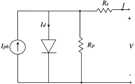
The Lambert W-function is used to find a mathematical equation capable of describing the behavior of a photovoltaic model, including all related parameters. The Lambert w-function has been widely used in many publications and fields to reduce the complexity and describe the behavior of a photovoltaic system, by converting the nonlinear and complex equation into explicit form [5]. Figure 1 represents a photovoltaic model with a single diode; under illumination the relation between the current and voltage of the photovoltaic single diode is given by [6]:

where, Vth=K.T/q is the thermal voltage of the photovoltaic module; Iph is the irradiance current (photocurrent); I0 is the cell reverse saturation current (diode saturation current); q is the electron charge; n is the cell ideality factor; K is the Boltzmann constant; T is the cell temperature; and Rs and Rp represent the cell series and shunt resistance, respectively.
The Lambert W-function is the inverse function of
f(w)=wew
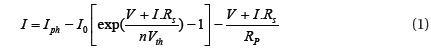
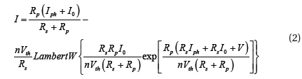
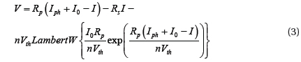
Equation (1) is transcendental in nature, and the explicit form
Similarly, the output power of the photovoltaic array can be given in explicit terms, as follows:
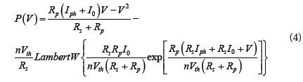
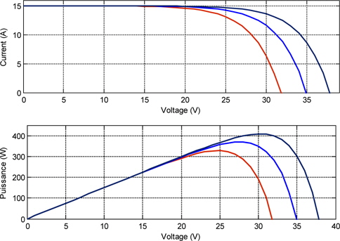
Figure 2 presents the characteristic current-voltage and power-voltage of the photovoltaic cell for different values of temperature and solar incident irradiance.
In the electrical characteristics, two points exist for a specific curve that can generate more power than other points. The maximum output power varies with temperature and irradiation change, so it necessary to extract the maximum available power for any changes.
3. STATE FEEDBACK MODEL OF THE THREE-PHASE PHOTOVOLTAIC
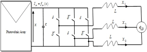
Figure 3 shows the general circuit topology configuration of a three-phase photovoltaic grid connected inverter connected to the grid connected to the inductance. The system is composed of a photovoltaic array, three-phase inverter and capacitive DC-link. The photovoltaic array converts solar irradiation into DC current, and the DC-link capacitor reduces the harmonic of the DC voltage on the input side of the inverter.
The three-phase inverter model of Fig. 3 given in states space coordinates by:
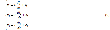
Park’s transformation is applied to equation (5)
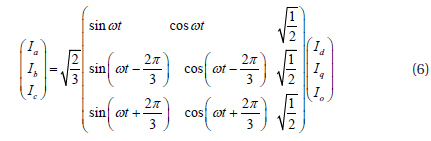
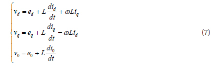
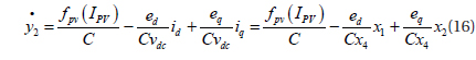
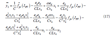
We apply the d-q transformation to equation (6), and obtain the state-space d-q in equation (7)

where, ed, eq, e0, id, i0, vd, vq and v0 are the components of the grid voltage, grid current, and inverter output voltage, respectively, and ω is the angular frequency. The power losses are neglected in inverter switches, and the power of the DC-input and AC-output is given by:

Where, vdc and idc are the input voltage and current of the inverter, respectively.
Kirchhoff’s law gives

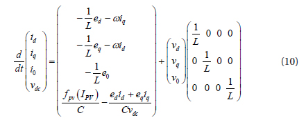
From equations (7) and (9), the equation of the state model can be grouped as:

3.1 State feedback linearization controller
The main objective of feedback linearization control is to transform and eliminate the nonlinearity model of the photovoltaic inverter system into a simple equivalent linear model, and find a direct relation between the output and the control input, by using inverse dynamics [7,8].
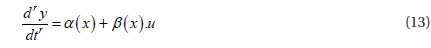
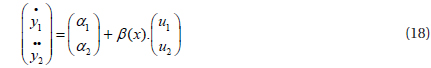
Let us consider a nonlinear control system of the phase state variable vector and phase input vector. The input-output state equation of the three-phase system is
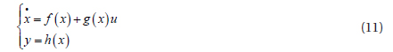
where,
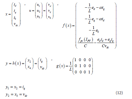
The outputs are differentiable until the inputs appear for searching for the exact input output. Let ri be a small integer such that at least one of the inputs appears in the ri th derivation of yi . The method is detailed in [9,10].

When
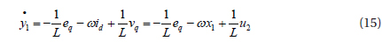
For the first output:

We have u2 input from the first derivation and the relative degree is r1=1.
For the second output:

The inputs u1 and u2 appear after the second derivation and the relative degree is r1=1.
The sum of r1+r2=3 and this is the order of the system. Then we can give an exact linearization of the system.
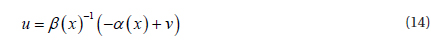
From equations (14) and (16), the feedback linearization of the system is
where:
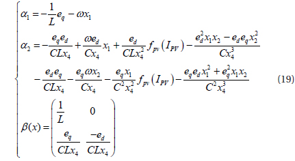
Where, β(x) is a non singular matrix, whose determinant is:

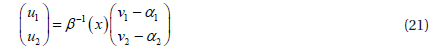
The corposant ed of the grid-connected voltage is always different from zero. Then the determinant is not null, and β(x) is nonsingular. The linearization of the control part is

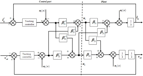
To eliminate the nonlinearity of the system, we substitute equation (21) into (18). So the simple linear relation between outputs yi and the new inputs vi is:
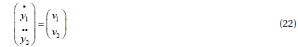
The nonlinearity of the system is cancelled, and Fig. 4 presents the linear equivalent control block diagram of the proposed method.
The controller is designed to obtain the stability of an integral controller, which is added to eliminate the steady-state error due to parameter variations.
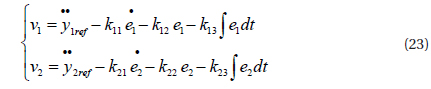
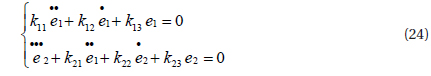
where, e1=y1−y1ref, e2=y2−y2ref and yref is the tracking error, y1ref is the tracking reference of the grid current reference, y2ref the DC-link voltage reference, and kij the gain. Then, the output error is:

The controller gains kij are determined by Rolls-criterion and to assure the characteristic polynomial of the equation (24), these are Hurwitz polynomials, so the error trackings of e1 and e2 converge to zero.
4.1 Conventional PID controller
The conventional fundamental classical PID controller is often described by the following equation in ideal form for the output voltage of a grid photovoltaic system [11-13]:

where, e1(t)=y1−y1ref, e2(t)=y2−y2ref and e3=(t)yref is the tracking error, in which Vout(t) denotes the controller output at time t of the photovoltaic array. Kp, Ki and Kd are known as the proportional constant, integral constant, and derivative constant respectively.
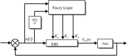
4.2 Structure of the PID-fuzzy self-tuning controller
Figure 5 shows the structure of the control system with the proposed PID-Fuzzy logic controller. The principle of fuzzy self-tuning PID is first to find the fuzzy relationship between the three parameters of PID and error ei (t)(i=1, 2 and 3) and the variation of the error (i=1, 2 and 3), and adjust the PID parameters with fuzzy rules. Fuzzy inference engines modify three parameters, to be content with the online demands of the control system. The inverse reference model of the response of the controlled object is used in the approach to tuning the PID-fuzzy controller.
The input parameters are the deviation ei(t) and the variation of deviation Δei(t), which are shown in equation (26). The output is the variation of MPPT.
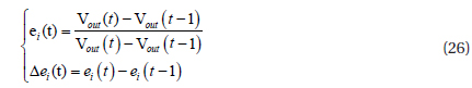
The output parameters are Kp, Ki and Kd, and continuously detect ei(t) and Δei(t) according to the fuzzy logic rules and regulations in order to satisfy the desire of the two inputs to the parameters of the controller at any time [14].
According to the methodology proposed by Zhao [15], the three current PID parameters are determined as follows. We assume the range of Kp is [Kp,min Kp,max], the range of Ki is [Ki,min Ki,max], and the range of Kd is [Kd,min Kd,max]. The range of Kp and Kd can be normalized into the range, through the linear transformation in equations (27) and (28).
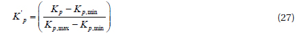

where, K'p, K'd, and α are constants that are determined by means of the fuzzy mechanism. The Kp,min, Kp,max, Kd,min, Kd,max are constants adopted to normalize the values of Kp and Kd which are given by :


The parameters Kp, Ki , and α are determined by a set of fuzzy rules.
If ei(t) is Ai and Δei(t) is Bi, then K'p is Ci , K'd is Di, and α=αi (i=1, 2…m). Here, Ai, Bi , Ci, and Di are fuzzy sets on the corresponding supporting sets, while αi is a constant.
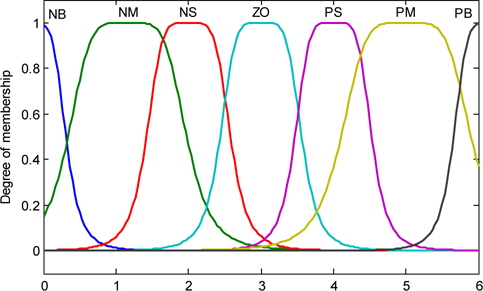
The fuzzy rules variables values of the input ei(t) and Δei(t) are configured for seven membership functions with NB= Big Negative, NM=Medium Negative, NS=Small Negative, ZO=Zero, PS= Small Positive, PM=Medium Positive, and PB=Big Positive, in the format of fuzzy control rules:
{NB, NM, NS, ZO, PS, PM, PB}
with the truth value of {0,6}
Figure 6 shows the memberships of the input variables ei(t) and Δei(t).
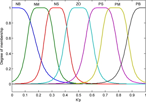
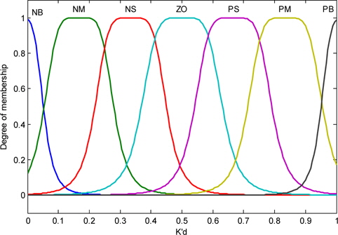
The output K'p and K'd use two exponential membership functions; to calculate K'p and K'd, we need to correct the factors K'p and K'd in the range. The values of the linguistic variable of K'p and K'd are shown in Figs. 9 and 10.
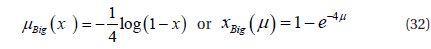
The fuzzy sets Ci and Di may be either Big or Small and are characterized by the grade of the membership functions μ, and the variables μ=(K'p or K'd) have the following equations:
For Small:

For Big:
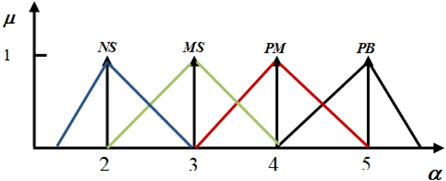
To calculate the integral coefficient Ki , correction of the factor is needed, and considered as a fuzzy number, it has a singleton membership function represented by points in Fig. 9, and has 7 linguistic variables, whose values are {α..NB, αNM, αNS, αZO, αPS, αPM, αPB}, their value being 2, 3, 4, 5.
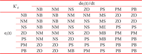
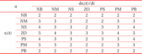
Through the analysis of the characteristic curve of a photovoltaic array, we can track the fuzzy control rules and correction factor of the classical PID controller parameter, for which ei(t) and Δei(t) are in different conditions. The fuzzy control rules are shown in Tables 1, 2, and 3.
[Table 1.] The fuzzy control rules for K'p.
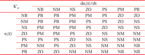
The fuzzy control rules for K'p.
[Table 2.] The fuzzy control rules for K'd.

The fuzzy control rules for K'd.
[Table 3.] The fuzzy control rules for α.

The fuzzy control rules for α.
Theoretical analysis of the proposed hybrid control of the output current and voltage of the three-phase photovoltaic system is validated and done by simulation using the Simulink platform. The simulation started when the solar irradiance was at G=1,000 W/m² and T=25℃. Firstly, the three-phase grid-connected photovoltaic inverter using the proposed hybrid controller is studied, in comparison with the separated classical PID controller. The inverter is connected to the DC source through a DC-link capacitor, with constant voltage reference value used to emulate the output of the maximum power point controller. The DC-link capacitor voltage is regulated and controlled by a PID-Fuzzy logic control loop, to reduce the oscillation in Pr at twice the line frequency due to grid imbalances. The output is the reference power, which must be injected into the grid by the inverter. The simulation control of the sinusoidal output current and voltage obtained with the DC-link capacitor replaced by a constant voltage source Vlink=400 V. The objective is to analyze the behavior of the current and voltage controller of Figs.10, 11, and 12, without influence of the DC-link and of the rest the system.
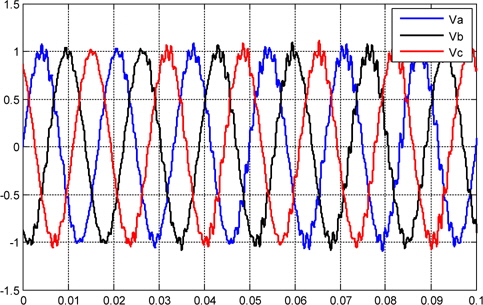
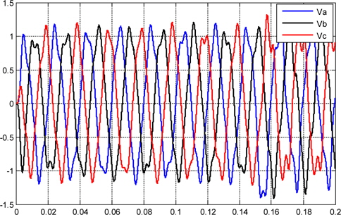
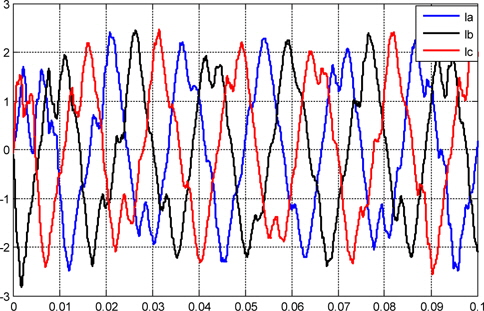
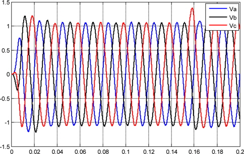
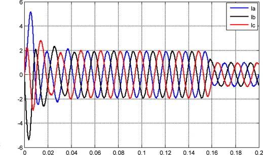
Figures 10, and 11 show the current and voltage, respectively, that are synthesized by the PID controller, and injected into the grid. Figure 14 shows the plot voltage at the load.
Due to the structure of the three-phase photovoltaic system converter, the output current and voltage are disturbance and unbalanced operating condition as shown in Figs.10,11, and 12.
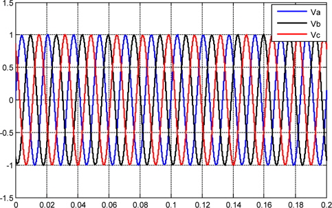
The objective now is to present the results of the simulation with all system parts of the photovoltaic array and DC-AC converter working together, relative to the PID-fuzzy controller.
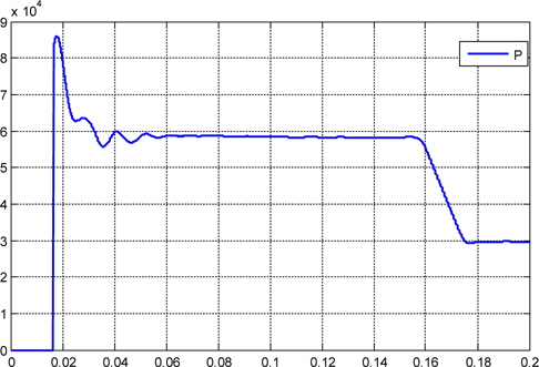
From t = 0 s to t = 0.16 s the system drains energy from the AC grid. From t = 0.16 s, the converter injects active power into the grid. At 0.16 seconds the reference current is stepped, and after this time, the converter operates in a steady state condition. Overall, the controller provides an excellent dynamic response.
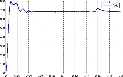
Figure 16 shows the behavior of the DC-link voltage, which initially is not charged. The photovoltaic capacitor is charged from 0 V to 700 V from the photovoltaic array. During the initial charge, the photovoltaic array supplies its maximum current, approximately near 0.16 s; and when the capacitor is charged, the DC-AC starts to supply current to the grid. The output sinusoidal current draining power to charge the capacitor suffers a phase inversion near t=0.16 s, and from this time, the DC-AC converter begins to deliver active power to the grid, as in Figs. 14 and 15.
This paper presented an intelligent hybrid based on PID control, and a fuzzy logic controller was proposed to control and stabilize the three-phases of the output current and voltage of the photovoltaic grid-connected converter. The system is complex and nonlinear, and a Lambert W-function and feedback linearization method was proposed. In the analysis, a fully mathematical approach was used to gain insight into the behavior of the photovoltaic model related to the one-diode equivalent circuit. The feedback linearization method and state feedback law transform and eliminate the nonlinearity model of the three-phase photovoltaic into a simple linear model. Nowadays, it has become evident that complex and nonlinear problems need intelligent systems to be solved. Recently, more than 95% control loops still use the PID controllers. They are used with fuzzy logic control to overcome the problems in the unknown mathematical model of the system. A PID-Fuzzy logic hybrid controller was applied to the control power system. Furthermore, fuzzy logic controller is implemented as a gain scheduler to automatically tune the Kp, Ki and Kd parameters for the PID controller. The system was regulated and controlled, and the results show the active power reduced in oscillation, and the current and voltage stabilized. As the results confirmed, initially the DC-link voltage capacitor is not charged, and during the charge, the three-phase photovoltaic system supplies a maximum current; and when the capacitor charges, the DC-AC starts to supply the grid. Compared with conventional controllers, this ensures minimum peak values in the grid-injected currents during unbalanced voltage sags. The proposed intelligent hybrid controller gave fast response and stability without delay, eliminating the oscillation around the operating points. From the simulation results, we concluded that the performance of the intelligent controller is better than the ones obtained with the classical PID controller, since the response time in the transitional state was shortened, and the fluctuations in the steady state were considerably reduced.