Radar has been developed in automotive sensor systems since the 1970s because of its long range, accuracy, and adaptability in all-weather conditions. Initially, the key idea of the automotive radar system was collision avoidance; however, many different applications of the vehicle radar system are now under development [1]. For example, convenience equipment, such as adaptive cruise control (ACC), has already been commercialized. Applications of the safety system for autonomous driving are the major topics of current radar research [1,2].
One of the requirements for radar of an autonomous driving system is a high-resolution capability, which is very difficult for the small-sized automotive radar because angular resolution directly depends on the antenna aperture size. However, parameter estimation methods by an array antenna can overcome this limitation of size. Multiple signal classification (MUSIC) is a well-known array processing method for high-resolution angular estimation [3-5], and its applications are being extended to various areas [6-9]. In this method, angle resolution is independent of the aperture size with ideal assumptions, such as uncorrelated signals, high signal-to-noise ratio (SNR), and large samples [10,11].
Unfortunately in practice, as in automotive radar systems, these assumptions cannot be satisfied because of the highly correlated signals, low SNR, and small number of snapshots. Research efforts have attempted to overcome these limitations; most of these are de-correlation methods based on preprocessing schemes, such as forward/backward (FB) averaging or spatial smoothing (SS) [12]. In another approach, beamspace MUSIC (BS-MUSIC) has been studied to improve radar performance in low SNR conditions. Several studies have reported that BS-MUSIC has advantages of low sensitivity to system errors, reduced resolution threshold, and improved performance in environments with spatially colored noise [13-17].
In this paper, we focus on increasing the number of snapshots by applying sawtooth waveforms. We show that this waveform enhances the angular estimation capability of MUSIC in addition to its well-known advantages of removing the ambiguity of the targets and improving velocity resolution. Despite these advantages, sawtooth waveforms have not often been used because of their high computational power. However, due to advances in digital technology, such as the digital signal processor (DSP) and FPGA, we can now implement signal processing units, including sawtooth waveforms and FBSS BS-MUSIC, which is one of the high-resolution angle estimators.
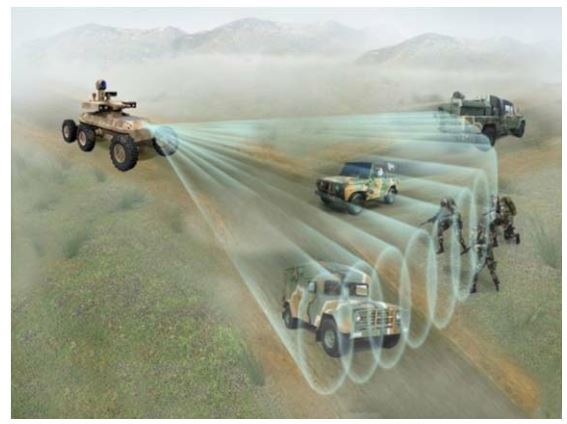
In cooperation with the Korea Agency for Defense Development, we developed a 77-GHz FMCW radar sensor as part of the sensor system for the defense unmanned ground vehicle (UGV) or robot, which is designed to run on unpaved or bumpy terrain, such as mountain roads. Fig. 1 shows the operational concept of the radar in a UGV.
Compared with commercial automotive radar, UGV radar must be capable of detecting slower targets in a harsh cluttered environment, covering wide angular sections in an azimuth up to 120°, and resolving targets with high angular resolution at the same time. In order to meet these requirements, we applied sawtooth waveforms in our process and designed the system using array antennas, an FPGA-based preprocessor for digital beam forming (DBF), and DSP for complex signal processing and high-resolution angle estimation.
This paper is organized as follows: Section II describes our FMCW radar sensor and the signal processing method, including waveform design and high-resolution angle estimation. Section III shows the experimental results with simulated data as well as measured data. Conclusions are presented in Section IV.
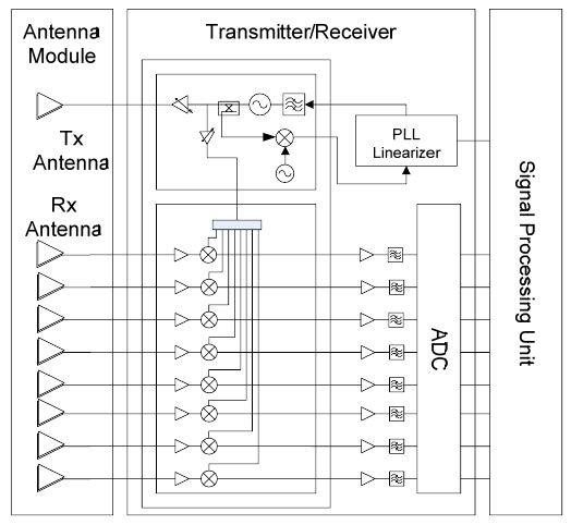
The radar system consists of antenna devices, transmitter/receiver, and the signal processing unit, as shown in Fig. 2. The transmitter/receiver has a homodyne structure. One broad illuminating transmitting beam and eight receiving beams overlap in the azimuth to yield a total azimuthal coverage of 60°. DBF was developed by using these eight received signals. The 3-dB beamwidth after DBF is about 15°. Some specifications of the transmitter/receiver are listed in Table 1.
[Table 1.] Specifications of the transmitter/receiver
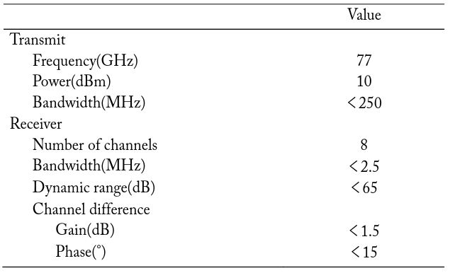
Specifications of the transmitter/receiver
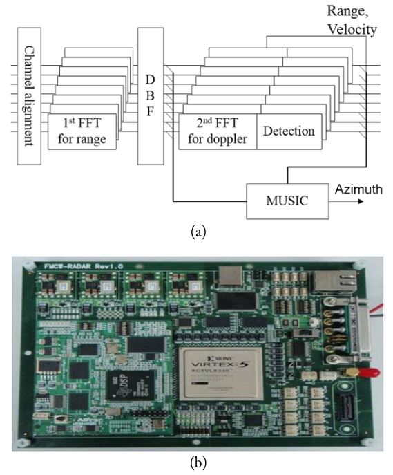
Due to the impairments of the radio frequency (RF) frontend, the signal vector is distorted and degrades the resolution. Thus, the first process after converting the input to a digital signal is channel alignment by a pre-measured calibration matrix. Each data signal is transferred to the frequency domain through first FFT for extracting the range information according to the FMCW principle. Then, the corrected signals are transferred to the beam space via DBF. Because of the sawtooth waveform, a second FFT is necessary to extract velocity information; this will be explained in the next section. The resulting data from the second FFT, which is called the range-Doppler map, are used to detect the targets via the constant false alarm rate (CFAR) method. After this main detection process, MUSIC is performed with some information in advance. The whole block diagram is shown in Fig. 3(a).
Since various computations of DBF, FFT, and MUSIC are included in signal processing chains, we designed our board using Virtex-5 FPGA (XC5VLX330; Xilinx Inc., San Jose, CA, USA) and DSP (TMS320C6455; Texas Instruments, Dallas, TX, USA) in order to make a real-time system. The preprocessing part including channel correction and DBF is implemented in FPGA, and the detection and FBSS BS-MUSIC are implemented in DSP. Fig. 3(b) shows our signal processing board.
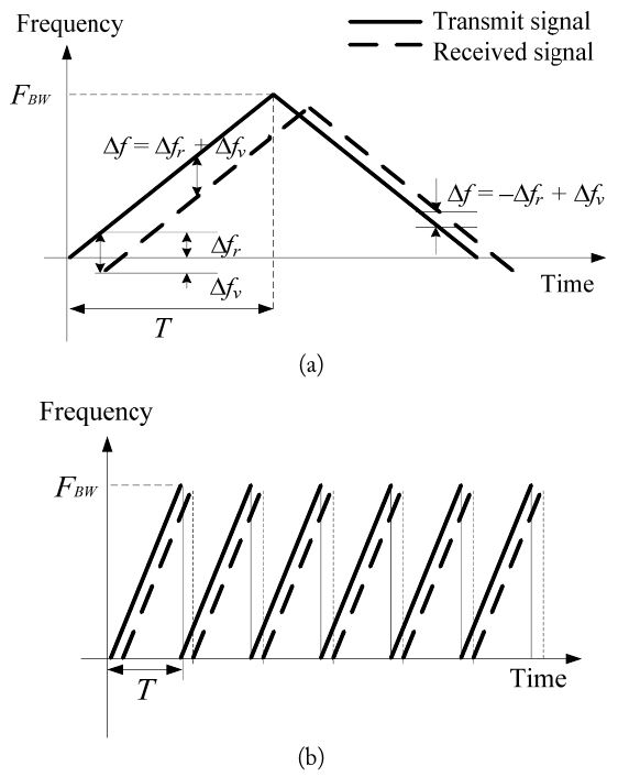
In the FMCW principle, targets are detected using the difference in frequency between transmitted and received signals, as shown in Fig. 4(a). This difference is due to the range and the velocity of targets. Each frequency difference by range (Δ
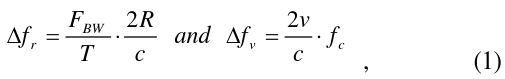
where
As the slope increases, usually by decreasing
Although the sawtooth waveforms might require more elaborate design work and much more computational power, it improves performance of detection for multiple targets with more velocity resolution, which is necessary for slow-movingtarget detection in a cluttered environment. Moreover, this burst of ramps improves the performance of high-resolution estimation, a main interest in this paper, by giving more snapshots. The computational power is no longer challenging, considering the advances of FPGA and DSP technology.
The parameters used in this paper are
3. High-Resolution Estimation Algorithm: FBSS BS-MUSIC
Consider a uniform linear array consisting of M identical sensors and
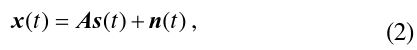
where s(

with
If the beamforming matrix is

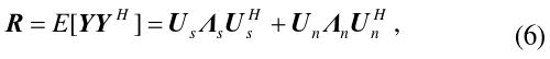
then the covariance matrix is

where
and that it corresponds to a target direction of angle (DOA).
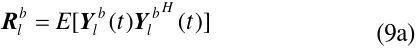
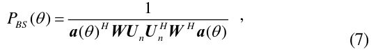
We apply the FBSS method in [12] as the configuration of Fig. 5. The covariance matrix of the


where
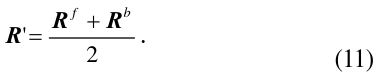
The FB smoothed covariance matrix

Replacing

where
If
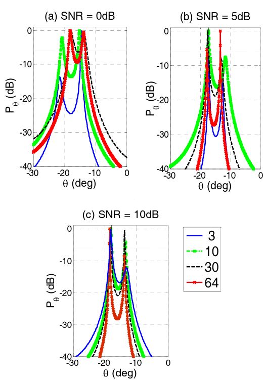
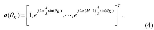
In order to see the effect of the number of snapshots, i.e., sawtooth waveforms, a set of received signals on arrays from two targets at -14° and -18.5° was simulated with random noise. Shown in Eq. (4), the signals were simulated based on the equal and omnidirectional element pattern. Although we verified the effect with white Gaussian noise, we used the colored noise in this simulation because it shows the effect clearly and is more realistic. The colored noises are generated by random noises passed through a filter. Based on the SNR, they were amplified and added to the signals.
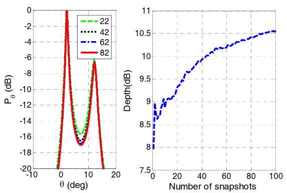
The normalized angular spectrums with different SNRs are shown in Fig. 6. As the number of snapshots increases, two peaks from the targets sharpen so that the two targets can be more easily resolved. In addition, the estimated angles approach the true values.
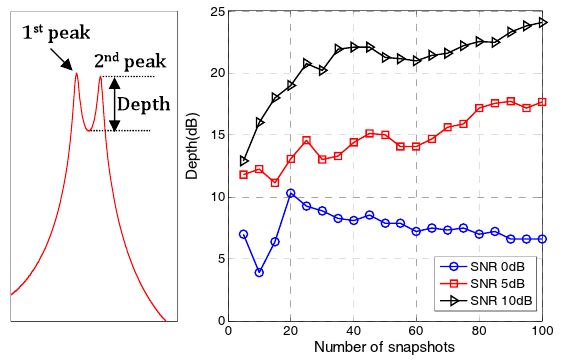
The sharpness can be represented by the depth, which is defined as the value of the second peak from the valley between two peaks. The depth increases as the number of snapshots increases if the SNR is ≥5 dB, as shown in Fig. 7.
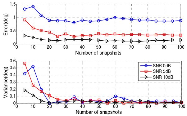
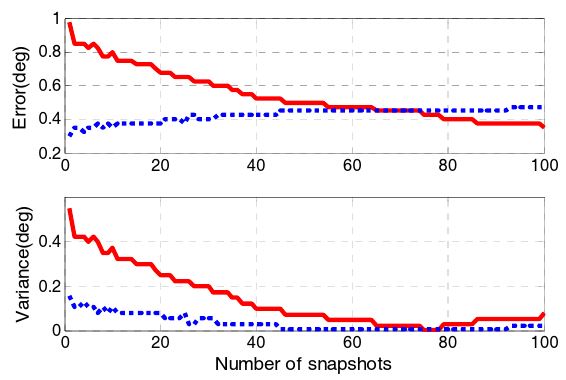
In addition, the number of snapshots improves the error performance. Fig. 8 shows the angle errors with respect to the number of snapshots for different SNRs.
As the number of snapshots increases up to 20 in this case, the estimated errors decrease and converge to a single value for each SNR. This bias error decreases as SNR increases. Moreover, the variance of errors is reduced continuously as the number of the snapshots increases for all SNRs.
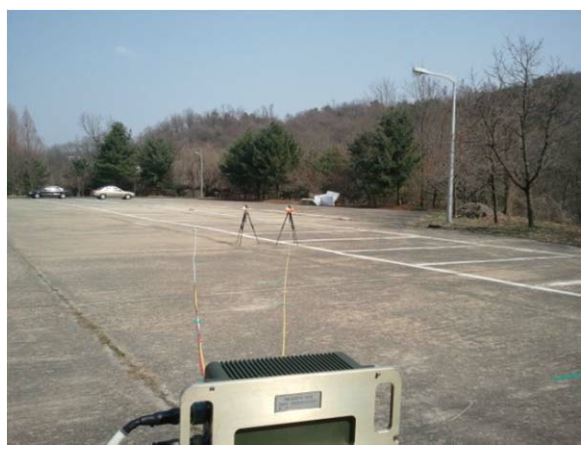
In the experiment to verify the method, we used two corner reflectors, as shown in Fig. 9. The reflectors were located at 2.4° and 11.5°, respectively, from the bore sight of the radar. The angle difference was about 60% of the beamwidth.
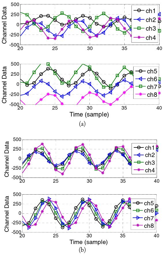
First, using a premeasured calibration matrix, each channel data record were aligned, as shown in Fig. 10.
The resulting depth and errors are shown in Figs. 11 and 12, respectively, with respect to the number of snapshots. The estimated errors are reduced to less than 0.5° in bias and 0.1° in variance by using more snapshots.
We implemented a real-time radar system of the high-resolution angle estimation for a UGV. We designed sawtooth waveforms and applied them with DBF and FBSS BS-MUSIC in signal processing units using FPGA and DSPs. The experimental results showed that two targets apart in less than 60 % of the beamwidth are resolved in real-time processing. We also showed that more snapshots from sawtooth waveforms improve the accuracy and the robustness for the high-resolution angle estimation