Many concepts for the commercial production of deep-seabed manganese nodules have been studied from the 1970s (Brink and Chung, 1982; Chung, 1996; Herrouin et al., 1989; Amann et al., 1991; Liu and Yang, 1999; Hong and Kim, 1999; Deepak et al., 2001; Handschuh et al., 2001). The accumulate ground of the deep-seabed has a problem, in that the bearing capacity of the ground is not strong, because the accumulate ground is formed by fine particles with high moisture content. So it is impossible to carry manganese nodules in the collection system. Therefore, the validity of continuous mining by lifting pipe from ground to vessel is highly appreciated.
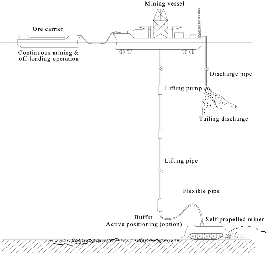
A continuous mining system is composed of mining vessel, lifting pipe, buffer system, transfer tube (flexible pipe), and self-propelled mining robot. The shape of the transfer tube between the buffer system and mining robot has a big impact on the driving efficiency of the mining robot. Also, the relative position between the buffer system and mining robot influences the efficiency of the mining robot. So, dynamic analysis of the integration of the mining system (mining vessel-lifting pipe-buffer system-flexible pipe-mining robot) is a very important technique in building a deep-sea mining system.
Currently, the lifting pipe and the flexible pipe are actively studied, according to the growth of offshore plant and the ocean floor industry. But studies on the buffer system are at an early stage. Just several functions to temporarily store nodules were mentioned by researchers (Chung, 2003; Kotlinski et al., 2008).
The coupling device of the buffer system is the main subject of this study. The buffer system is currently developing. This coupling device makes a big impact on the dynamic movement of a mining robot. And it is a very important mechanic device in a deep-seabed mining system. The specs of the coupling device are determined by various efficiency tests and changes of design. But the production and experiment of a buffer system is costly and time-consuming. So the design specs of this device must be found by simulation. In general, this design method is called the simulation-based design.
Dynamic analysis of mechanical systems using computers is rapidly performed through the growth of computing power. The method of simulation-based design is a useful technique in otherwise impossible cases, which is verified by using an experiment with a model as an integrated deep-seabed mining system. The simulation technique is an excellent means of understanding qualitative (or quantitative) optimization design, and can skip the process of test model production, which is costly and time-consuming.
The mining robot and vehicle model used in this study is an MBD model. This MBD model was developed by Kim (Kim et al., 2010). The integrated simulation model is developed by DAFUL (2012).
In this study, the used equations are the joint constraints, a beam elastic equation and a multi-body dynamic solution. The verifications of the joint constraints and the beam elastic equation are written in DAFUL verification manual (2012).
In this study, joint constraints (Haug, 1989) were applied to find optimum kinematic characteristics of the coupling device. The joint constraints are as follows.
Fixed constraint
A fixed constraint can remove motion for all degrees of freedom of rigid bodies or flexible bodies. Eqs. (1) and (2) show the fixed constraint equations (Haug, 1989).


where,
Eq. (1) means a positional constraint, and Eq. (2) means a rotational constraint between the base body and action body. Eq. (1) is equal to a spherical constraint.
Revolute constraint
A revolute constraint is able to allow rotation between two bodies about one rotation axis. Eqs. (1) and (3) show the revolute constraint equations (Haug, 1989).

where,
Beam elastic theory is used to build flexible pipe and transfer tube. Euler and Timoshenko had verified the beam method using beam stiffness. The equation of beam stiffness is as in Eq. (4).
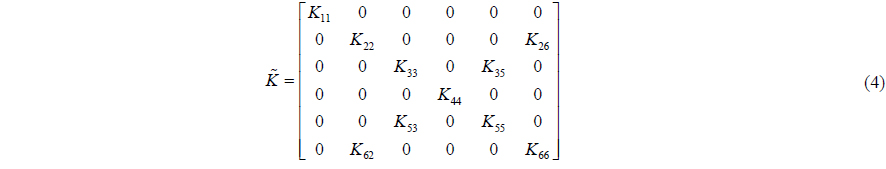
The beam stiffness matrix is a symmetric matrix. The components are as follows.


where,
The calculated stiffness is applied to the matrix force in DAFUL (2012). This matrix force can apply forces of 3 translational and 3 rotational directions in a rigid body. These forces are dependent on the displacements and velocities of element bodies.
All mechanical systems are composed as an assembly of many objects. This assembly has been called a multi-body. Multibody solutions are different from basic dynamic solutions. Multi-body solutions must find dynamic responses of each object, and exact solutions must be obtained by applying components, which are in correlation. Each body is defined to calculate the dynamic responses of a multi-body. The method to define an object is in two ways. First, an orthogonal coordinate system is attached to each body, and a motion of the body coordinate system is expressed by a generalized coordinate system. Second, connected bodies in series are numbered in couplers of the multi-body.
The body’s equation of motion is defined as a differential equation. The multi-body system’s equation of motion has nonlinearity of relative coordinate, velocity and acceleration.
An eidetic method to change from nonlinearity to linearity is that the equation is expressed by only the relative coordinate, velocity and acceleration. And relative coordinates must be expressed as equations of independent coordinates, velocities and accelerations. An interaction formula between an independent coordinate and dependent coordinate is able to lead from a constraint equation of position, velocity and acceleration.
The equation of motion is defined as follows (Haug, 1989). A multi-body system can be modeled as a generalized coordinate of ‘ngc’ dimensions. These generalized coordinates are expressed as Eq. (13). Also, the velocity and acceleration coordinate are defined as Eqs. (14) and (15) respectively.


If a system has independent constraint equations of ‘


where a is the acceleration vector of rigid bodies, and Φ
The equation of motion for a multi-body system having constraint is as in Eq. (18).

where M is the mass matrix,
The equation of motion about the system is changed as a matrix, using Eqs. (17) and (18).

The position, velocity and acceleration of a rigid body can be solved by these.
DYNAMIC MODEL OF DEEP-SEABED MINING SYSTEM
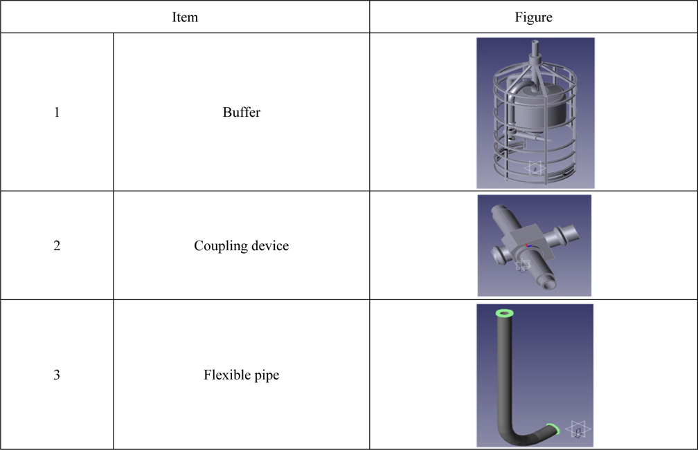
A buffer system is a mechanical structure to save collected mineral lumps. A mass of the buffer system is 8
[Table 1] Components of buffer system.

Components of buffer system.
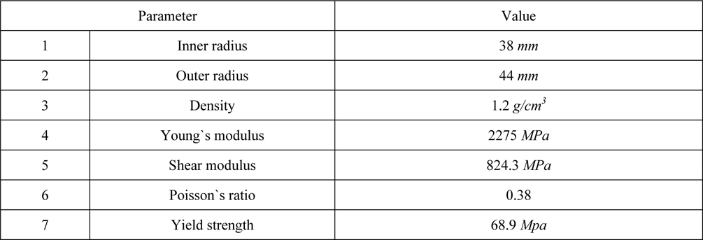
A flexible pipe in a buffer system provides passage to transfer minerals. The pipe that has generally been used is a PVC (polyvinyl chloride) pipe. The characteristics of the PVC pipe are given in Table 2.
[Table 2] Characteristics of PVC pipe.

Characteristics of PVC pipe.
The buffer and coupling device are built as a rigid body, to neglect the material deformation.
1) A swivel joint is built between the buffer and ground. The swivel joint is used to constrain the buffer’s rotation. Components of the swivel joint are the revolute joint and stopper. In this study, the stopper is built using a rotational spring damper and stiffness coefficient by the curved radius of the buffer. Also, the effect of the vessel is applied to the buffer.
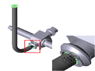
2) Three constraints are used to research the kinematic characteristic of the coupling device between the flexible pipe in the buffer and the coupling device. They have 6 D.O.F, 5 D.O.F, and 3 D.O.F. Fig. 2 shows their constraints.
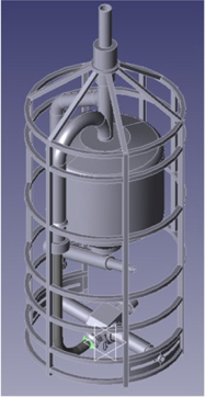
A buffer system model to perform numerical analysis is developed as in Fig. 3.
>
Integration simulation model of mining system
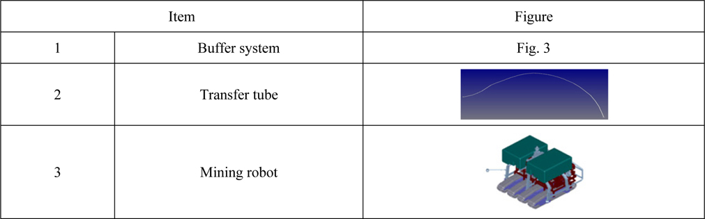
An integration model is built with the buffer system model, mining robot and transfer tube. They are shown in Table 3. The mining robot model is developed as in the Kim’s last study (Kim et al., 2010). The transfer tube is built by beam elastic theory, to advance solving time. In common, dynamic responses by the beam model are equal to the results by the finite element method. But the solving time is very fast. The characteristics of the transfer tube are shown in Table 4.
[Table 3] Components of the integration simulation model.

Components of the integration simulation model.
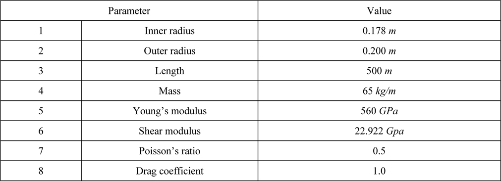
[Table 4] Characteristics of the transfer tube.

Characteristics of the transfer tube.
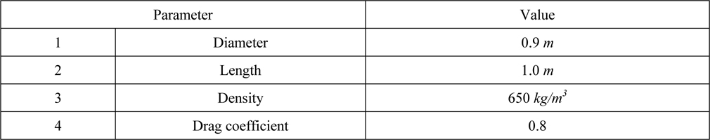
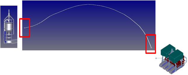
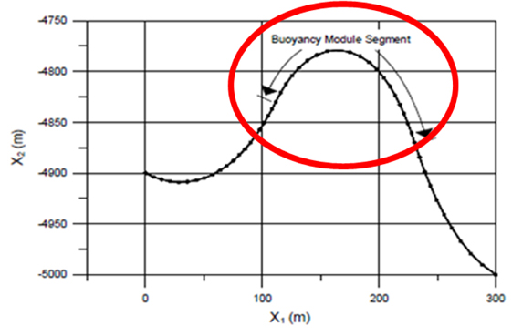
This transfer tube is affected by the fluid drag force, owing to its long length. So the drag force must be applied to the tube. Buoyancy modules are provided to prevent twisting and bending at particular positions of the transfer tube in the seabed environment. The characteristics of the buoyancy module are shown in Table 5, and the positions of the buoyancy module are shown in Fig. 4.
[Table 5] Characteristics of the buoyancy module.

Characteristics of the buoyancy module.
Also, the inner flows generate in the pipe. The inner flows are a very complex chaotic phenomenon. Many studies are required to analyze the impact between nodules, the momentum change, the contact phenomenon between nodules and wall of the inner pipe and the expansion of compressed air. But the forces by inner flows are much smaller than the external forces. When we design the structures the effects of inner flows are not considered due to this reason. So in this study, inner flows are not applied.
The equation of the fluid drag force is as follows.

where
The buoyancy equation is as follows.

where
Fig. 5 shows the developed integration simulation model.
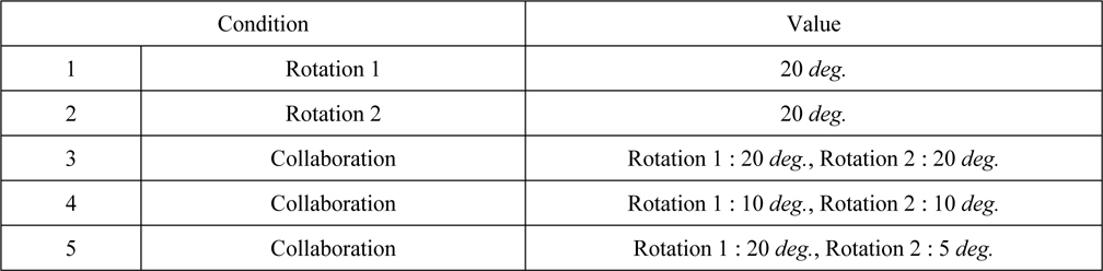
Forced motion is the basic test condition to estimate loads. The test conditions for movements of the coupling device are as follows.
[Table 6] Forced motion condition.

Forced motion condition.
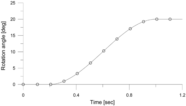
A maximum rotation angle of the coupling device for design is 20
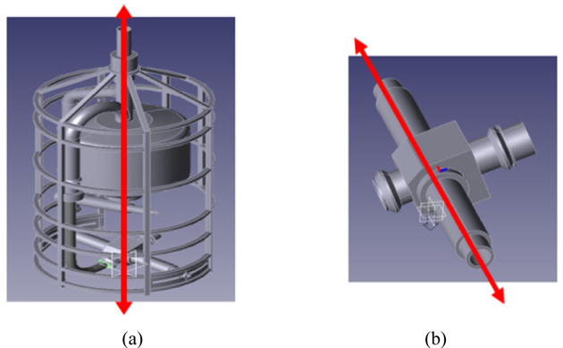
The rotation axes of conditions 1 and 2 are shown in Fig. 7.
Total simulation time is 1.2
When the vessel and mining robot are driven, motions of the coupling device may be different from the results of the forced motion condition. Load estimation about the combined model must be performed. But the driving effect of the vessel is applied to the buffer system. Its effect is irrelevant to the movement of the coupling device. And the solving time is advanced, due to it being a simple model.
In this study, the driving conditions of the vessel and mining robot are determined by the results of Brink (1981), and Hong and Kim (2008). Detailed driving conditions for the load estimation are shown in Table 7.
[Table 7] Driving conditions for load estimation.
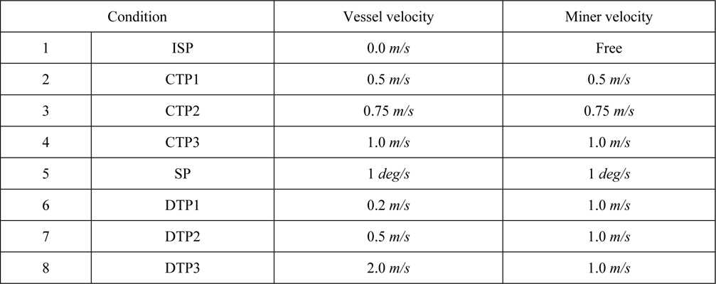
Driving conditions for load estimation.
NUMERICAL RESULT AND LOAD ESTIMATION
>
Load estimation by forced motion
Condition 1
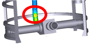
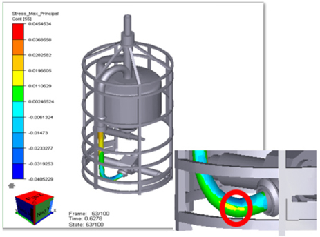
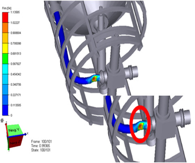
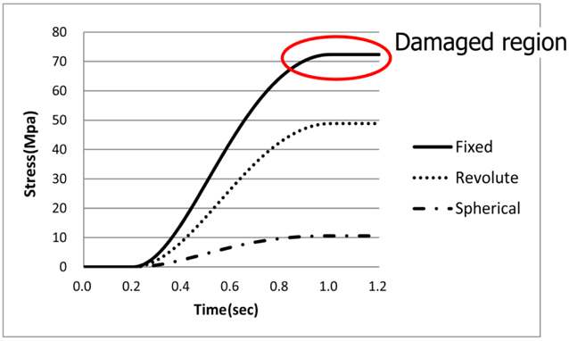
Loads are estimated at the position of maximum stress and load in the flexible pipe. In figures, the color means size of stress. The red color is maximum stress of the pipe and the blue color is minimum stress. The position is shown in Fig. 8.
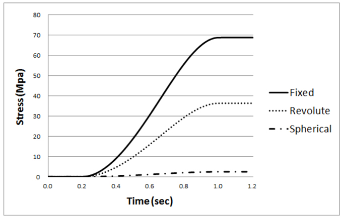
Measured loads of the flexible pipe are different according to the kinematic constraints in condition 1. The loads are as follows.
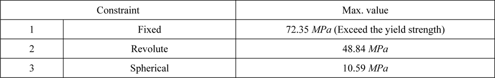
[Table 8] Maximum load of flexible pipe in condition 1.
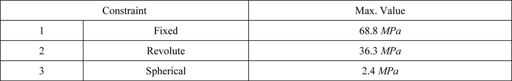
Maximum load of flexible pipe in condition 1.
In fixed constraint, stress of pipe has come close to the yield strength. But other cases have not come close to the yield strength. When the coupling device has a rotational degree of freedom, the stability of the flexible pipe is better than with no rotation.
Condition 2
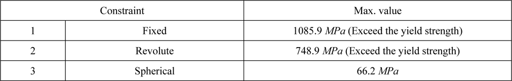
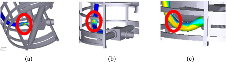
Loads are estimated at the position of maximum stress and load in the flexible pipe. The position is shown in Fig. 10.
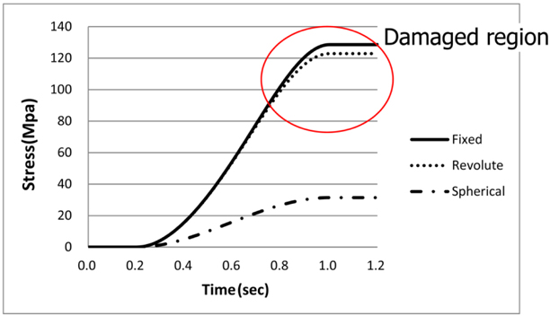
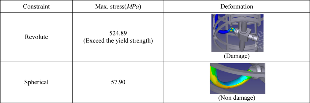
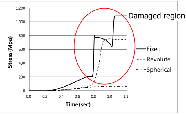
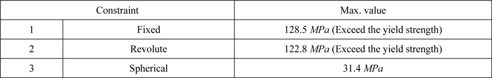
The measured loads of the flexible pipe are different according to the kinematic constraints in condition 2. The loads are as follows. The loads in fixed & revolute constraints are exceeded the yield strength. These facts mean the breakdown of flexible pipe. When the kinematic constraint is fixed constraint, the load of the pipe has bigger than revolute constraint. And the tendency of load has been dramatic changes. Also, the revolute constraint has bigger than spherical constraint. This means that rotational degree of freedom is very important for safe design.
[Table 9] Maximum load of flexible pipe in condition 2.

Maximum load of flexible pipe in condition 2.
We knew that deformations of the flexible pipe differ according to kinematic constraints of the coupling device. Fig. 12 shows their deformations. When the coupling device has rotational degrees of freedom, the load of the flexible pipe is smaller than with no rotation. Snapping of the pipe did not occur, so the mineral can be transferred easily. Also, when this device has 3 D.O.F for rotation, the stress of the flexible pipe keeps within the yield strength.
Condition 3
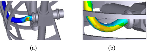
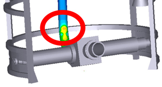
In this case, measurement positions for the load estimation are not the same, because the maximum load and stress are applied by constraints at different points. The positions are shown in Fig. 13.
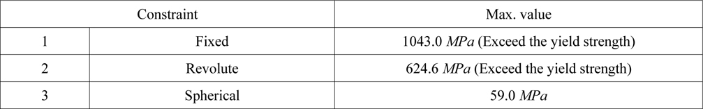
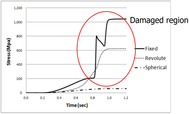
The measured loads of the flexible pipe differ according to the kinematic constraints in condition 3. The loads are as follows. The tendency of results is similar to the condition 2. This means that rotational degree of freedom is very important for safe design in condition 3.
[Table 10] Maximum load of flexible pipe in condition 3.

Maximum load of flexible pipe in condition 3.
The result by fixed joint is much larger than the result by spherical joint. This result shows that the structural stability differs according to the kinematic characteristics. And the bending phenomenon is expressed in the fixed joint and revolute joint. But it is not expressed in the spherical joint. Therefore, the fixed joint of kinematic characteristics is a very bad constraint. So result analysis by fixed joint is excluded in the integration analysis.
Condition 4
Loads are estimated at the position of maximum stress and load in the flexible pipe. The position is shown in Fig. 15.
The measured loads of the flexible pipe differ according to the kinematic constraints in condition 4. The loads are as follows. The tendency of results is not similar to the condition 2. This means that the motion of rotation axis 2 had given a significant effect on the load.
[Table 11] Maximum load of flexible pipe in condition 4.
Maximum load of flexible pipe in condition 4.
In fixed and revolute constraints, stress of the pipe has come close to the yield strength. But spherical constraint has not come close to the yield strength. When the coupling device has rotational degrees of freedom, the stability of the flexible pipe is better than with no rotation.
Condition 5
Loads are estimated at the position of maximum stress and load in the flexible pipe. The position is shown in Fig. 17.
The measured loads of the flexible pipe differ according to the kinematic constraints in condition 5. The loads are as follows.
[Table 12] Maximum load of flexible pipe in condition 5.

Maximum load of flexible pipe in condition 5.
In fixed, stress of the pipe has come close to the yield strength. But other constraints have not come close to the yield strength. When the coupling device has rotational degrees of freedom, the stability of the flexible pipe is better than with no rotation. Also, we can know that the rotational degree of freedom by rotation 2 is very critical parameter to prevent damage.
>
Load estimation by driving motion
The load results for each driving condition are as follows.
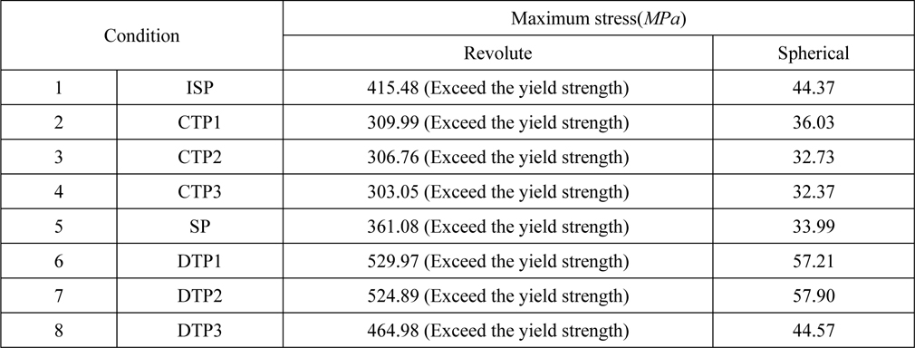
[Table 13] Load estimation by driving condition.

Load estimation by driving condition.
In all conditions, the spherical joint is better than the revolute joint. And when kinematic characteristic is spherical constraint, the stress of pipe doesn`t exceed the yield strength. This result shows that the rotational degree of freedom is a very important parameter in the design of a coupling device.
In DTP1 and DTP2 driving conditions, the loads of the flexible pipe are distinguished according to their kinematic characteristics. It is known that the driving velocities of the vessel and mining robot are important. Research into this behavior will be conducted in the future.
[Table 14] Load estimation in DTP1 of driving condition.

Load estimation in DTP1 of driving condition.
[Table 15] Load estimation in DTP2 of driving condition.

Load estimation in DTP2 of driving condition.
Through this study, a concept of the simulation-based design by using multi-body dynamics is introduced through the kinematic design of the buffer system. The results of this study are as follows.
1) Kinematic design of the coupling device of the buffer system
The loads of the flexible pipe depend on the kinematic characteristics of the coupling device. The size of the loads as follows.
Fixed constraint >> Revolute constraint >> Spherical constraint
When the coupling device has many the rotational degrees of freedom, the load of the pipe is very small. This result shows that the rotation of the coupling device is dominated with the stability of buffer system. Thus, the rotational degree of freedom is very important design parameter for the buffer system design.
The bending and twisting of the flexible pipe do not appear when there is the rotational degree of freedom. This enables the stable transfer of the minerals. And only, the result of the spherical constraint is not exceeded the yield strength in all conditions. The coupling device that has the rotational degrees of freedom must be produced for stable transfer of mineral and the stability of the buffer system. Also, we can be known that the rotational degree of freedom is a factor affecting equipment stability in operation of the vessel and the mining robot.
2) Simulation-base design
We can be known that the simulation-based design is the useful design process for a producing of deep-seabed equipment. The simulation-based design method is based on the multi-body dynamics, the nonlinearity is considered. For this reason, this design method considers influences by motions and forces of the actual equipment.
Yet, the theory on the simulation-based design is not formulated perfectly.
Finally, the potential of the simulation-based design is confirmed in this paper. In the future, we will formulate the theory of the simulation-based design method and design other mechanic systems of deep-seabed mining system by using the simulation-based design.