The visualization of partially occluded 3D objects has been considered one of the most challenging drawbacks in the 3D-vision field [1, 2]. To solve this problem, several multiperspective imaging approaches, including integral imaging and axially distributed image sensing (ADS), have been studied [3-9]. Integral imaging uses a planar pickup grid or a camera array. On the other hand, an ADS method, implemented by translating a camera along its optical axis, was proposed to take digital plane images that can be refocused after elemental images (EIs) have been taken for 3D visualization of partially occluded objects [10-14]. This method provides a relatively simple architecture to capture the longitudinal perspective information of a 3D object.
However, the capacity of the ADS method is related to how far the object is located from the optical axis. Due to a lower capacity for objects located close to the optical axis, wide-area elemental images are needed to reconstruct better 3D slice images under a large field of view (FOV).
In this paper, in order to capture a wide-area scene of 3D objects, we propose axially distributed image sensing using a wide-angle lens (WAL). Using this type of lens we can collect a lot of parallax information. The wide-area EIs are recorded by translating the wide-angle camera along its optical axis. These EIs are calibrated for compensation of radial distortion. With the calibrated EIs, we generate volumetric slice images using a computational reconstruction algorithm based on ray back-projection. To verify our idea, we carried out optical experiments to visualize a partially occluded 3D object.
In general, a camera calibration process is needed for the images captured with the camera mounted with a WAL. Therefore, to visualize the correct 3D slice images in our ADS method, we introduce a camera calibration process to generate calibrated elemental images. This camera calibration method has never been applied to the conventional ADS system.
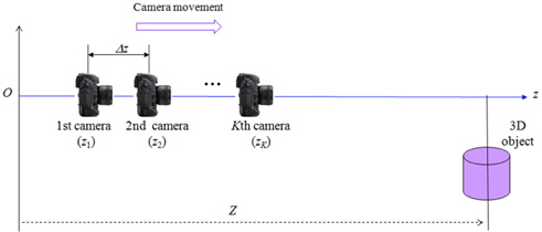
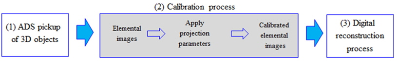
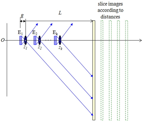
Figure 1 shows the scheme of the proposed ADS system with a WAL. It is composed of three different subsystems: (1) ADS pickup, (2) a calibration process for elemental images, and (3) a digital reconstruction process.
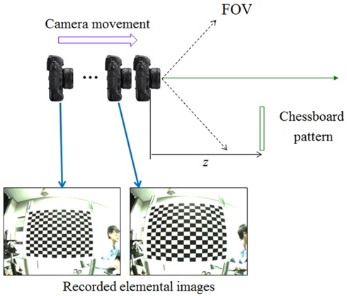
The ADS pickup of 3D objects in the proposed method is shown in Fig. 2. Compared to the conventional method, the camera mounted with a WAL is translated along the optical axis. Let us define the focal length of the WAL as
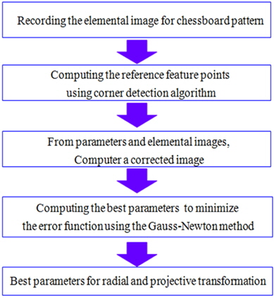
In a typical imaging system, lens distortion usually can be classified among three types: radial distortion, decentering distortion, and thin prism distortion [15]. However, for most lenses the radial component is predominant. We assume that our WAL produces predominantly radial distortion, and ignore other distortions in a recorded image. Therefore, the image distortion should be corrected by a calibration process before the digital reconstruction used in the proposed method. Our calibration process is composed of two steps. In the first step, the radial distortion model is considered. We suppose that the center of distortion is (
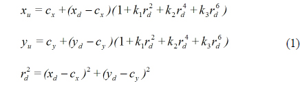
From Eq. (1) we can see that the distortion model has a set of five parameters
In the second step, the point with coordinates (
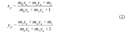
Here, it is seen that the projection parameters are
Before recording 3D objects, we want to find the two parameter sets
2.3. Digital Reconstruction Process
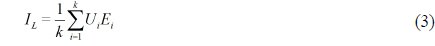
The final process of our wide-angle ADS method is digital reconstruction using the calibrated EIs described in Section 2.2. In this process we generate a slice-plane image according to the reconstruction distance. Figure 5 shows the digital reconstruction process based on an inverse-mapping procedure through a pinhole model [7]. Each wide-angle camera is modeled as a pinhole camera with the calibrated EI located at a distance

where
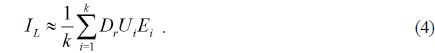
To reduce the computational load imposed by the large magnification factor, Eq. (3) is modified by using the downsampling factor

In Eq. (4)
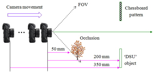
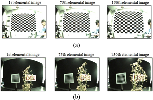
We performed preliminary experiments to demonstrate our proposed ADS system for partially occluded object visualization. Figure 6 shows the experimental structure we implemented. As shown in Fig. 6, we used two scenarios at the same time. The first scenario has a single object with a chessboard pattern with square size 100 mm × 100 mm. The second scenario has two objects: a tree as the occluder, and ‘DSU’ letter objects with letter size 100 mm × 70 mm to demonstrate partially occluded object visualization. The chessboard pattern and ‘DSU’ are located 350 mm from the first wide-angle camera position, as shown in Fig. 6. The occluder is located 150 mm in front of the ‘DSU’ object.
We use a 1/4.5 inch CMOS camera with a resolution of 640 × 480. The WAL has a focal length
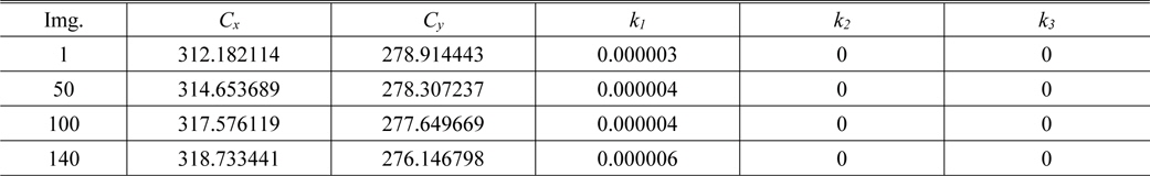
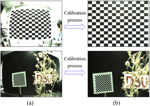
After recording the EIs using the wide–angle camera, we applied the calibration process to them. Each EI was corrected using the corresponding calibration parameters. The calculated parameters are shown in Tables 1 and 2 for the radial distortion and projective transformation (
[TABLE 1.] Computed parameters Θd for radial distortion

Computed parameters Θd for radial distortion
[TABLE 2.] Computed parameters Θp for projective transformation
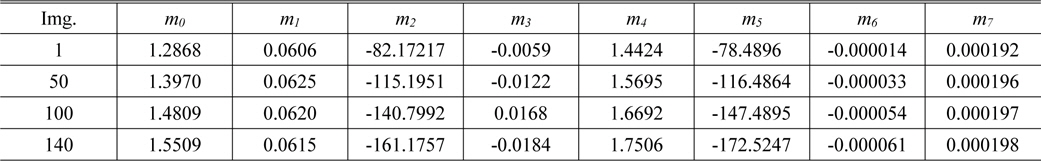
Computed parameters Θp for projective transformation
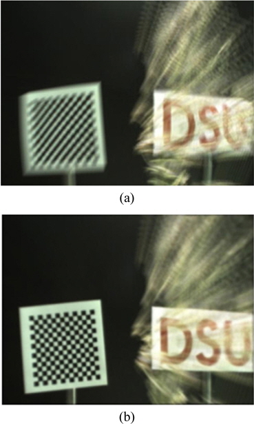
With the calibrated EIs as shown in Fig. 8, we reconstructed slice plane images for 3D objects according to the different reconstruction distances. The 150 calibrated EIs were used in the digital reconstruction algorithm employing Eq. (2). The slice image at the original position of the 3D objects is shown in Fig. 9. For comparison, we include the results of using the conventional ADS method without a calibration process. From the experimental results, we can see that our method can be demonstrated successfully for visualizing a partially occluded object.
In conclusion, we have presented a wide-angle ADS system to capture a wide-area scene of 3D objects. Using a WAL we can collect a lot of parallax information for a large scene. The calibration process was introduced to compensate for the image distortion due to the use of this type of lens. We performed a preliminary experiment of partially occluded 3D objects and demonstrated our idea successfully.