Recently there has been considerable interest in spectral reflectivity recovery methods in the field of color science [1-7] because of their fundamental importance, as well as their technological significance. In general, the color of an object is determined by the illumination conditions and the reflectivity of the surface material [8-10]. The light spectrum reflected by the material is passed through the eye and quantified by tristimulus values [8-10]. The spectral behavior of a colored object is known to be the fingerprint of the color, which is independent of the applied light source and the observer (for nonfluorescent materials). Spectral reflectivity recovery is also important for multispectral image processing, color consistency, color reconstruction, and color image processing [1-3].
Recovering the spectral reflectivity from known tristimulus values is an inverse problem for a given illumination condition [1, 7, 8]. In general, the solution to such an inverse problem is ill-posed, meaning that an exact and accurate solution is not easy to find. The solution also depends on the noise and initial conditions [11-13]. Two major methods for spectral reflectivity recovery are the pseudo-inverse technique [2-6, 14-17] and the interpolation technique [7, 18-20]. In the pseudo-inverse technique, principal-component analysis [2-6, 14-16] and nonnegative matrix transformation [7, 17, 21-23] are developed with various adaptation techniques. These are partially successful at reflectivity recovery, but finding an appropriate adaptation set requires extensive computation time, and the adaptation algorithm itself suffers from a localization problem.
A three-dimensional (3D) interpolation technique is often applied to minimize calculations when approximating mathematically defined complex functions, or to produce intermediate results from sparse data points [11, 24]. Both situations can be directly employed when we convert images from one device-dependent color space to another, or invert a color space to reflectivity data [1, 7, 18, 20]. Nearest neighbors with given tristimulus values and reflectivity data are needed to obtain the reflectivity of the target tristimulus values. 3D interpolation with Delaunay tetrahedration extracts the four vertices of a tetrahedron and calculates the reflectivity value of an unknown point inside. The 3D interpolation technique is faster, in terms of computational time, than other methods [1, 7, 18, 20, 24]. However, the interpolation technique can only be applied to find the tristimulus values of points that are inside the color gamut of a training data set [7, 18, 20]. The tristimulus values of a point outside the color gamut (convex hull) of the training set cannot be interpolated.
In our previous study [7] we applied a hybrid method for spectral reflectivity recovery, interpolating tristimulus values when the data are inside the color gamut, and using nonnegative matrix transformation (NMT) when the data are outside. This technique has overcome the color gamut problem of the interpolation method and is faster than previous pseudo-inverse techniques. However, even with this fast and effective hybrid method, out-of-gamut data still must be recovered through the time-consuming pseudoinverse technique of NMT. In this report, we apply a simple extrapolation technique [11, 24-27] to the spectral recovery process to address the color gamut problem of interpolation. We start with a brief introduction of the 3D Delaunay interpolation method and proposed algorithms for the 3D extrapolation of tristimulus values. Next, four different algorithms for obtaining the vertices of a tetrahedron are presented and used for 3D extrapolation. We analyze the statistics of the extrapolation technique in terms of efficiency, accuracy, and color difference. Finally, we present a comparison between this extrapolation method and various pseudo-inverse techniques.
The 3D interpolation technique has been used in various fields to deal with scattered data [1, 7, 11, 18-20, 24]. It has also been applied to spectral reflectivity recovery, and is regarded as a fast and reliable method [7, 18, 20]. In this section, the concept of the 3D interpolation technique is revisited and summarized. This technique will be extended to a 3D extrapolation technique, explained in Section 2.2.
The reference color data points are usually given by CIE

The coefficients
In a 3D interpolation technique, the reflectivity value

In Eq. (3) the four coefficients

In the 3D interpolation algorithm, the four coefficients of color matching range between 0 and 1. Implementation of the 3D interpolation algorithm requires the following five steps:
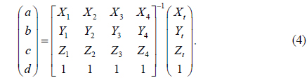
1. Calculating CIE XYZ data from given reflectivity data and other conditions. 2. 3D Delaunay triangulation of data points. 3. Finding a tetrahedron that contains target CIE XYZ data. 4. Calculating the barycentric coordinate of target CIE XYZ data using Eq. (4) and the four vertices of the tetrahedron. 5. Calculating the reflectivity value of the target point using Eq. (3).
Basically, color matching in additive mixing is a linear and additive problem, as shown by Eqs. (1)-(3). The 3D interpolation of reflectivity involves a simple, linear technique. However, there are two points to be considered. First, spectral recovery is an inverse problem with many possible solutions. The spectral value of the target point is determined by the characteristics of neighboring points. Depending on the reference data set, a completely different reflectivity with the same CIE
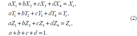
In this section we develop a simple 3D extrapolation [11, 24-27] that can be applied to spectral-recovery problems. We reconsider the interpolation problem by examining some basic equations, Eqs. (1)-(4). The barycentric coordinate equation of Eq. (4) is the main equation of 3D interpolation. Its limiting condition is that the four coefficients,

The corresponding reflectivity matching equation (Eq. (3)) is then

The meanings of Eqs. (5) and (6) can be interpreted as follows. To obtain the reflectivity of a target color
It is essential for implementation of this extrapolation algorithm to find an appropriate tetrahedron for the calculation of the barycentric coordinates. One still can utilize the strategy of 3D interpolation. We tested four different algorithms to define tetrahedra for extrapolating color data. The first choice in defining the tetrahedron is finding the four nearest neighbors of the target color point. Then the Euclidian distance between the target point and reference can be calculated, and a neighbor-searching algorithm can be applied to define four points from which to construct a tetrahedron.
The next choice in defining the tetrahedron is the utilization of information from the 3D interpolation. In our 3D interpolation we used the Delaunay tessellation algorithm in MATLAB® (version 7.11, MathWorks) [24]. In mathematics and computational geometry, [11, 24] a Delaunay triangulation for a set P of points in a plane is a triangulation DT(P) such that no point in P is inside the circumcircle of any triangle in DT(P). Delaunay triangulation maximizes the narrowest angle of all angles of the triangles in the triangulation. Therefore, the circumcenters of all tetrahedra have already been calculated by 3D interpolation. We used the circumcenters of partitioned tetrahedra and calculated the Euclidian distances between the circumcenters and the target point to find an appropriate tetrahedron of neighbors. One can also calculate and tabulate in-centers and centroids of tetrahedrons by 3D Delaunay tessellation. We applied three methods (circumcenters, in-centers, and centroids) with given tessellation information to define a tetrahedron, and the neighbor-searching algorithm was applied to find an appropriate tetrahedron. After finding an appropriate tetrahedron, the four coefficients of mixing can be calculated easily by modifying the algorithm for 3D interpolation.
The reflectivity spectra of 1269 color chips from the Munsell color matte finish collection book were downloaded from a website [28] and used as a reference data set. The original reflectivity data were measured using a spectrophotometer (Lambda 18, Perkin Elmer), the wavelengths of the data ranging from 380 to 800 nm with intervals of 1 nm. In this work the reflectivity data from 400 to 700 nm with intervals of 10 nm were used to evaluate the proposed reconstruction algorithm. A spectral reflectivity recovery algorithm was developed, which includes the process of rebuilding the reflectivity through a hybrid method using 3D interpolation and 3D extrapolation. To calculate a CIE
To evaluate the proposed algorithm, the mean and maximum root-mean-square errors (RMSE) between the original and reconstructed reflectivity spectra were evaluated. We have examined the significance of the reconstructed reflectivity data using the coefficient of correlation (COC) [12, 29] as follows:
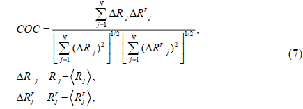
where
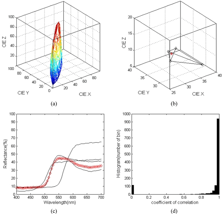
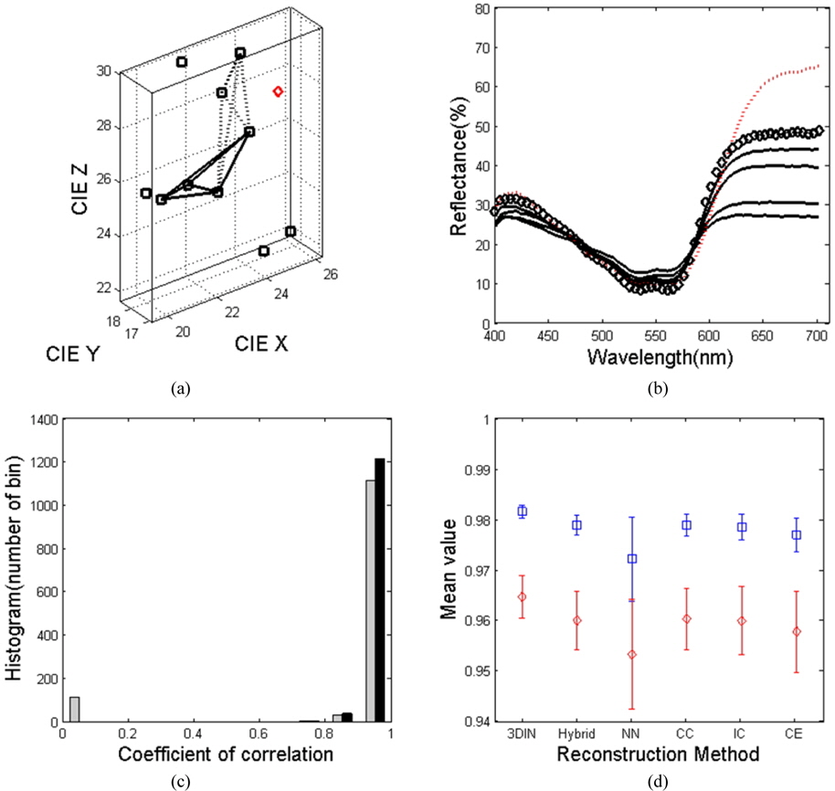
Figure 1(a) shows the color gamut and 3D Delaunay tetrahedrization results of 1269 Munsell color chips in CIE
This recovery procedure was repeated for all 1269 Munsell colors, and coefficients of correlation are depicted in Fig. 1(d). It is extremely difficult to reconstruct some of the reflectivity data because they belong to the border between different color chips, for which interpolation will have considerable uncertainty [7, 18, 20]. As previously discussed, 115 data points define the convex hull of the 3D CIE
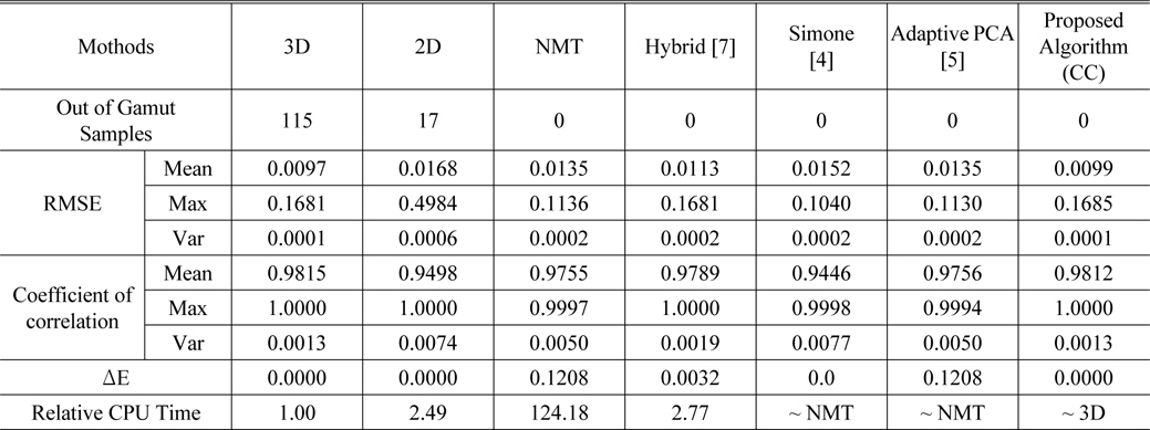
Statistical summary of various reflectivity reconstruction methods applying 1269 Munsell color data
When the target data points are outside the gamut of the reference reflectivity data, fast and accurate 3D interpolation cannot be applied. Various techniques can be applied in such cases: different versions of principal-component analysis (PCA) and nonnegative matrix transformation (NMT) have been applied to the spectral recovery of “outside color gamut data” [2-7, 14-20]. In Table 1 we report the statistical values for various PCA and NMT techniques, as well as for our interpolation technique. The interpolation for inside-gamut data can be performed in 2D CIE
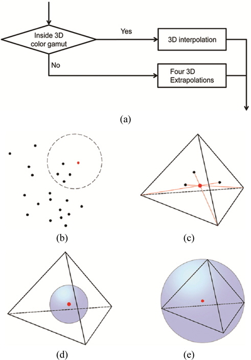
As described in Section 2, we implemented four different techniques for 3D extrapolation. Our basic algorithm for spectral recovery is shown in Fig. 2(a). The first implementation found the four nearest neighbors of the target data (shown in Fig. 2(b)), and we calculated the Euclidian distance between the target and neighboring data [32] and selected the four nearest data points for the spectral reconstruction. The next class of implementation involved using various properties of the tetrahedron that were already partitioned by 3D Delaunay tetrahedrization. Figures 2(c)-(e) show the centroid, in-center, and circumcenter of the tetrahedron respectively. The centroid of the tetrahedron is the arithmetic mean of its four vertices. The circumcenter and in-center are the centers of the circumsphere and in-sphere, respectively, which can be easily found using the built-in functions “circumcenters” and “in-centers” of MATLAB [11, 13, 24]. These points can be calculated and tabulated when the reflectivity data are given, so the additional computational time required for 3D extrapolation using these points can be minimized. It is worthwhile to mention the following points: First, the centroid and the in-center of a tetrahedron always lie within the tetrahedron, but the circumcenter may not. Second, a Delaunay tetrahedrization algorithm is based on circumcenters, the importance of which will be demonstrated later.
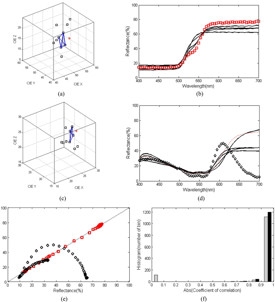
Having developed the 3D extrapolation techniques, we now describe the details and statistics of these techniques. The results of extrapolating nearest neighbors are shown in Fig. 3. Figures 3(a) and (b) show the spectral reflectivity recovery of the Munsell color 7.5YR 8/10 (#225), the circle in Fig. 3(a). This color belongs to the convex hull made by the 1269 Munsell reference colors and cannot be recovered by 3D interpolation. The four nearest neighbors of 7.5YR 8/10 are 10YR 5/8, 10YR 5/6, 2.5Y 8.5/10, and 2.5Y 8.5/8, plotted as a tetrahedron in Fig. 3(a), and their mixing coefficients in the 3D extrapolation are 0.8870, 1.1033, -0.0467, and -0.9435 respectively. Four reflectivity spectra are plotted as solid curves in Fig. 3(b), and the recovered spectrum is plotted as diamonds, while the original spectrum of 7.5YR 8/10 is depicted as a dotted curve. The spectral recovery of 7.5YR 8/10 is excellent. Figures 3(c) and (d) show the recovery of the Munsell color 2.5RP 5/12 (#1163). The four nearest neighbors are identified as 2.5RP 5/10, 10P 5/10, 10P 5/12, and 2.5RP 5/8, and they are marked as a tetrahedron; their mixing coefficients are 3.1520, 1.9981, −2.0704, and −2.0798 respectively. The recovered spectrum (diamonds in Fig. 3(d)) and original spectrum (dotted curve) do not match well. This disagreement could be a consequence of the tetrahedron being too small in the CIE
Information from 3D Delaunay tetrahedrization can be used to obtain better recovery results. We used centroids, in-centers, and circumcenters of tetrahedra from 3D Delaunay tetrahedrization, and the results are summarized in Fig. 4. Figures 4(a) and (b) depict the spectral reflectivity reconstruction of the Munsell color 2.5RP 5/12 (##1163) (the same color shown in Figs. 3(c) and (d)) using the circumcenter algorithm. The circumcenters of all tetrahedra were calculated using the built-in MATLAB function, and the Euclidean distances between circumcenters and the target point were computed. The shortest-distance selection criterion for the tetrahedron is shown by solid lines. The tetrahedron with dashed lines is from the nearest-neighbor point (Fig. 3(c) versus Fig. 4(a)). The Munsell notations of the vertices of the solid tetrahedron are 2.5RP 5/8, 2.5RP 5/10, 10P 5/6, and 10P 5/8. Two of them (2.5RP 5/8 and 2.5RP 5/10) are the same points selected by the nearest-neighbor algorithm. The mixing coefficients for the four vertices are −0.5370, 1.5980, −0.3030, and 0.2419, smaller than those of the nearestneighbor selection algorithm (3.1520, 1.9981, −2.0704, and −2.0798). The spectral-recovery result is shown in Fig. 4(b). The reflectances for the four vertices are shown as solid curves. The target reflectance and the recovered reflectance are shown as dotted and diamond curves respectively. Compared to those from previous nearest-neighbor algorithms (shown in Fig. 3(d)), the recovered spectrum matches the target reflectance fairly well.
The statistics for circumcenter extrapolation hybridized with 3D interpolation are shown in Fig. 4(c). The coefficient of correlation for 3D interpolation is shown as a gray bar, and the coefficient for the circumcenter extrapolation is shown as a black bar. We note that there is no reflectance with a zero coefficient of correlation, which appears in the 3D interpolation algorithm due to the out-of-gamut problem. The statistics for the circumcenter extrapolation are better than those for the nearest-neighbor algorithm. The mean values and variations of the coefficient of correlation for different methods are summarized in Fig. 4(d) using square symbols. “3DIN” represents 3D interpolation, for which the statistics are calculated without out-of-gamut data (115 data points). “Hybrid” represents the hybrid technique with 3D interpolation and nonnegative matrix transformation (NMT) [7]. NN, CC, IC, and CE represent nearest-neighbor, circumcenters, in-centers, and centroid extrapolation, respectively. Another statistical value, the coefficient of determination, is computed for the different methods and is shown with diamond symbols. Among the four extrapolation algorithms, the CC, IC, and CE methods are better than the NN method because of 3D Delaunay tetrahedrization. The CC, IC, and CE methods show nearly comparable results com pared to the hybrid technique of 3D interpolation plus NMT for spectral recovery. The statistical analysis data are also derived, and summarized in Table 1. We note that the out-of-the-gamut problem of 3D interpolation can be overcome by our 3D extrapolation technique; however, the overall statistics for the out-of-gamut data are not as good as in the case of the 3D interpolation for inside-gamut data. CPU times for reconstruction are also summarized in Table 1. The relative time is the time normalized to the 3D interpolation method. The method of Simone and adaptive PCA take nearly the same amount of time as NMT, and the proposed algorithm takes nearly the same as 3D interpolation.
We now consider the merits of 3D extrapolation compared to NMT and PCA. First, 3D extrapolation with CC, IC, and CE uses 3D Delaunay tetrahedrization, which is well known for its superior efficiency. In addition, a fast and accurate mathematical algorithm is used with the 3D Delaunay method. Second, the time to compute the 3D extrapolation is minimal compared to the execution time of the adaptive versions of PCA and NMT. Since the CC, IC, and CE of a tetrahedron are computed and stored as a database or look-up table (LUT), the time required for 3D extrapolation is hardly greater than the time required for 3D interpolation, which is at least two orders of magnitude faster than the other reconstruction methods [4, 6, 7]. Finally, the color gamut of 3D interpolation can be extended by accumulating more reflectivity data for the LUT. Also, the measure of fitting accuracy can be enhanced by the quality and the quantity of the data in the LUT, because most of the errors of 3D interpolation and extrapolation techniques come from color samples near the border between two colors with different character.
The recovery of spectral data is important because the spectral reflectivity of a color is a fundamental index which is unchangeable, even if the appearance of the color is affected by the ambient environment or the observer's vision. We propose a 3D extrapolation technique with 3D interpolation based on the Delaunay tetrahedrization algorithm for reflectivity reconstruction from the tristimulus values of colors. A previous 3D interpolation technique using a barycentric algorithm is extended to 3D extrapolation using four points among the nearest neighbors. In the proposed procedure, a 3D extrapolation technique is used to find the tristimulus values of color data that exist outside the color gamut. We applied and analyzed four distinct nearest-neighbor searching algorithms using nearest points, and the tristimulus values of the CC, IC, and CE of a tetrahedron. Statistical analysis, the coefficient of correlation, and the coefficient of determination show that the results of the CC, IC, and CE methods yield accuracy as high as that of the pseudoinverse technique. However, the extrapolation technique is much faster than the pseudo-inverse technique in terms of processing speed. We believe that the proposed 3D extrapolation technique for spectral reflectivity reconstruction could advance color research and widen applications, including color consistency, color reconstruction, and color image processing.