Golden cuttlefish Sepia esculenta is a commercially important cephalopod species in Korea. They are caught mainly during their spawning season, from May to June, when adults migrate from deep water to the littoral zone along the southwest coast of Korea. Assessment of their population biomass has relied entirely on landings data from commercial fisheries using gill-nets, hand-jigs, traps, set-nets, and trawls. However, each of these fishing methods select different portions of the population, potentially biasing the assessment. During 2011 to 2013, about 3,207 metric tons (mt) of cuttlefish were landed annually; and about 662 mt (~21%) of these were caught in inshore gill nets (KOSTAT, 2014). The increased demand for cuttlefish in Korea has motivated resource managers to consider alternative sources of information about the cuttlefish stock in the inshore and coastal fishing grounds (Lee et al., 1998; Watanuki and Kawamura, 1999).

Towards the development of a fishery-independent acoustic method for surveying cuttlefish, the magnitude and variability in its acoustic target strength (TS) must be evaluated. TS is an indicator of the size of an acoustic target, and is used to convert measurements of echo energy to estimates of fish abundance. It is broadly known that TS varies with acoustic frequency, and fish species, size, and swimbladder volume (Love, 1971; Foote, 1985; Goddard and Welsby, 1986; Demer and Martin, 1995; McClatchie et al., 1996; Conti and Demer, 2003; McClatchie et al., 2003; Kang et al., 2005; Simmonds and MacLennan, 2005; Lee, 2006; Foote, 2012), but the literature is devoid of TS measurements and models for cuttlefish. Based on the literature, especially Love’s summary of fish TS (Love, 1969; 1971), we hypothesize that cuttlefish TS is principally dependent on the incidence angle of the acoustic pulse on the cuttlebone, which, for measurements with a vertical echosounder, would be naturally modulated by cuttlefish behavior, particularly tilt angle (θ), during their vertical migration and feeding. Cuttlefish TS is also likely a function of mantle length (L), and the size and shape of the cuttlebone. The goal of this study is to develop empirical relationships between mean TS and L for live golden cuttlefish S. esculenta at two frequencies, 70 and 120 kHz.

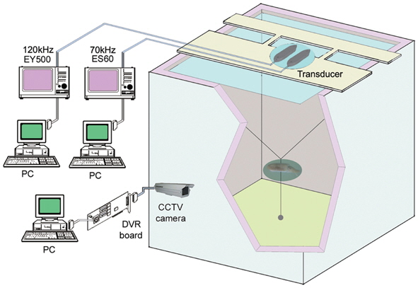
The acoustic and optical system for measuring the TS of live golden cuttlefish is shown in Fig. 1 (Lee, 2006). It is comprised of two echosounders (Simrad ES60 and EY500) operating at 70 and 120 kHz; two split-beam transducers (Simrad ES70-11 and ES120-7F; half-power beamwidths = 11˚ and 7˚, respectively); an apparatus to control the orientations of the cuttlefish; and a closed-circuit television (CCTV) camera (MIG System, KJ Tech, Korea) positioned outside of the transparent walls of the tank to continuously observe the fish locations, movements, and orientations during each acoustic transmission. A water-cooling system maintained the seawater at a temperature T = 18.7˚C (confirmed by measurements before and near the end of the experiment). The two transducers were mounted facing downwards, adjacently, with their faces approximately 10 cm below the water surface.

Before and near the end of the series of experiments, the 70 and 120 kHz echosounders were calibrated using copper spheres having diameters = 32.1 and 23.0 mm, respectively. The measured TS values were 0.3 dB lower and 0.5 dB higher than the theoretical values, TS_theory = -39.16 and -40.40 dB, respectively, for T = 13˚C and sound speed c = 1460 m sec^-1 (Simrad, 2003). The TS measurements were corrected for these calibrated offsets. During both the calibrations and the TS measurements, the 70 and 120 kHz echosounders transmitted 300 and 60 W pulses with 256 μs and 300 μs durations every 0.2 seconds, and received the echoes with 6.2 and 12 kHz receiver bandwidths, respectively.

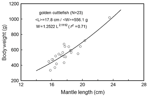
In early May 2010, 23 cuttlefishes were caught by traps in the inshore waters around Geojedo, Korea. Measurements of their mantle length (L) and body mass (W) ranged from 15.6 to 23.5 cm (mean L = 17.8; std = 1.8 cm) and 335 to 1,020 g (mean W = 556.1; std = 139.8 g), respectively. The conversion from cuttlefish length to mass is W = 1.2522 L^2.1112 (r² = 0.71, N=23) (Fig. 2). The cuttlefish were acclimatized to captivity in a small acrylic tank.

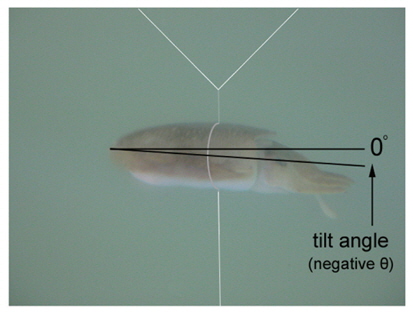
Before each set of measurements, a cuttlefish was tethered using two monofilament lines (0.2 mm diameter), each tied to the mantle of the cuttlefish body, and stabilized with a weight below (Fig. 3). Sequentially, each specimen was carefully lowered into the sound beams, avoiding the introduction of air bubbles. To avoid cross-talk between the echosounders and better position each specimen within each beam, the measurements at 70 and 120 kHz were made sequentially. In each case, the range between the transducers and the cuttlefish was ~1 m. The far-field ranges (r_ff = d²⁄ 2λ) for the f = 70 and 120 kHz transducers (d =13.5 and 12.9 cm) were ~0.47 and ~0.68 m (Lee, 2006; Foote, 2012), respectively. Following Foote (2012), the far-field range for the largest cuttlefish (L = 23.5 cm) was ~1.42 and ~2.27 m, respectively.

In succession, each cuttlefish was positioned near the beam axes by adjusting the tethers, guided by the CCTV images. When the echoes were relatively stable, TS measurements were recorded for approximately 5 min, for each frequency and fish. The echo data, logged by the echosounders, were post-processed using commercial software (Echoview V3.3, Sonar Data, Australia; and EP500 V5.2, Simrad, Norway).

The loosely tied cuttlefish were able to move some from the initial position. The CCTV images were recorded and later processed to estimate the tilt angle (θ) distributions.

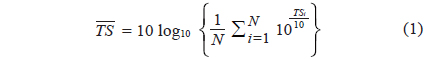
The mean TS for each cuttlefish at each frequency was estimated using:

where TS_i is the i_th measurement of TS, and N is the total number of TS measurements, for the specimen. To establish empirical, single-frequency relationships between the and corresponding L, the data for each frequency were fit independently, in the least-squares sense, to:

where L is the mantle length (cm), m is the slope of the regression line, and b is the intercept of the regression line on the axis. For fish, m is often assumed to be 20, indicating an areal dependence (Demer and Martin, 1995).

Then, the datasets from both frequencies were combined to obtain a relationship for a wider range of L and wavelengths (λ):

where L is the mantle length (m), λ is the acoustic wavelength (m) and a, b, c are fitted coefficients (Love, 1969; Love, 1971; Goddard and Welsby, 1986; McClatchie et al., 2003).

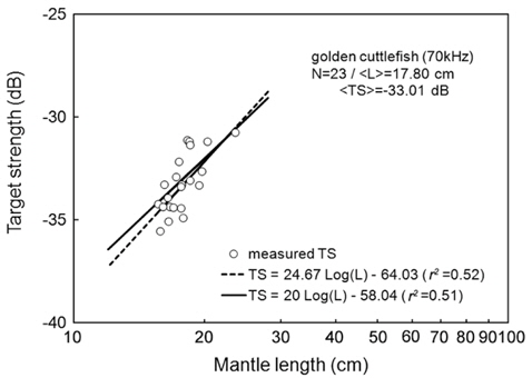
Separately for 70 and 120 kHz, the of 23 live cuttlefish were plotted versus L, overlaid on the regressions of Eq. (2) (Figs. 4 and 5), respectively. At 70 kHz,

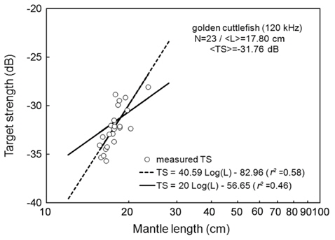
At 120 kHz,

The at 70 kHz was -33.01 dB, 1.25 dB lower than that at 120 kHz (-31.76 dB). The at 70 kHz was 0.17 dB higher than that indicated by Eq. (4a), and 0.02 dB higher than that indicated by Eq. (4b). The at 120 kHz was 0.45 dB higher than that indicated by Eq. (5a), and 0.12 dB lower than that indicated by Eq. (5b). The regression equations are significantly different at 70 versus 120 kHz, principally due to the large slope in Eq. (5a).

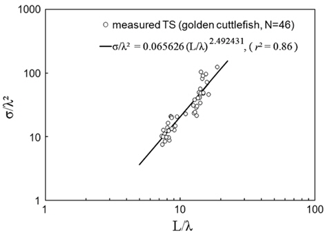
Combined for 70 and 120 kHz, the 46 measurements of were transformed to mean scattering cross-sectional areas (σ; m²) and σ²/λ was plotted versus L/λ (Fig. 6). In this wavelength-normalized form, the values for live cuttlefish are comparable between frequencies, allowing the following regression:

Transforming Eq. (6) to decibels and rearranging terms provides a model, in the form of Eq. (3), of versus L for individual cuttlefish:

where L is the mantle length (m), λ is the wavelength (m). The 95% confidence intervals (CI) for the regression coefficients [a, b, and c values in Eq. (3)] are 24.92 ± 3.08 (P < 0.01), -4.92 ± 3.08 (P < 0.01), and -22.82 ± 3.21 (P < 0.01), respectively. The values indicated by Eq. (7) are -33.23 dB at 70 kHz and -32.07 dB at 120 kHz. The differences between these values and the measured values are 0.22 dB at 70 kHz and 0.31 dB at 120 kHz.

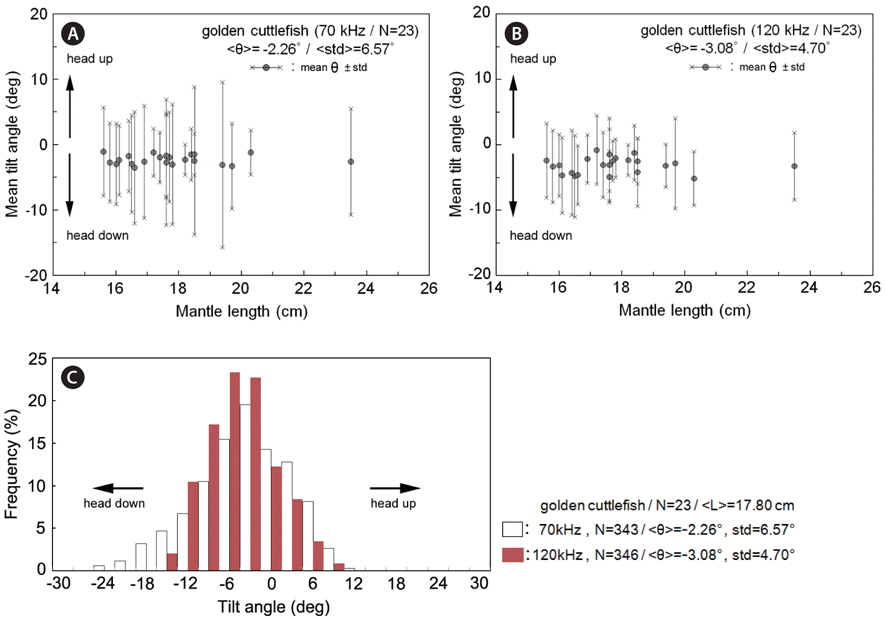
During the measurements of 70 kHz TS, the assumed-normal distributions of θ [N(mean, std)] were estimated for N=15 cuttlefish from 343 CCTV camera images captured at approximately 20 second intervals. Likewise, during the measurements of 120 kHz TS, the distributions of θ were estimated for N = 16 cuttlefish from 346 CCTV camera images. In both cases, the distributions of θ were strongly unimodal, ranging from -23.4˚ to 12.3˚ [N (-2.26˚, 6.57˚)] and -13.0˚ to 9.3˚ [N (-3.08˚, 4.70˚], respectively (Fig. 7). Positive θ indicates a head up orientation relative to the center line of the mantle or body, and a negative θ indicates a head down orientation. Although the standard deviation is larger for the tilt angles recorded during the 70 kHz TS measurements, the distributions are not significantly different.

An empirical relationship has been developed to estimate versus L for cuttlefish. This relationship [Eq. (7)] may be useful in analyses of data from acoustic surveys of cuttlefish off Korea, and perhaps elsewhere. Estimates of may be useful for acoustic estimations of fish lengths, but also to estimate fish biomass from measurements of echo energy.

Although the slope of a versus L relationship is often assumed to equal 20 [e.g., Eqs (4b) and (5b)], it may vary widely versus fish species (Love, 1969; 1971; Foote, 1985; Goddard and Welsby, 1986; Demer and Martin, 1995; Conti and Demer, 2003; McClatchie et al., 2003; Kang et. al., 2005; Lee, 2006). According to Simmonds and MacLennan (2005), the slope commonly has values between 18 and 30, although Kawabata (2005) reported a much smaller value (12.9) for ommastrephid squid. In this study, the slopes were estimated to be 24.67 ± 10.81 (P < 0.01) at 70 kHz and 40.59 ± 15.54 (P < 0.01) at 120 kHz, respectively [Eqs. (4a) and (5a)]. In other words, at 70 kHz, the of cuttlefish varies approximately as the square and fourth power of the mantle length at 70 and 120 kHz, respectively. These results suggest that the slope is significantly greater than 20 at 120 kHz, and the slopes are significantly different for different frequencies for the same species. The intercept of the regression line at 70 kHz, -64.03 ± 13.50 dB (P < 0.01), was 18.93 dB higher than that at 120 kHz, -82.96 ± 19.41 dB (P < 0.01).

The chi-square test of independence showed that the values for 23 cuttlefish at 70 and 120 kHz are independent (P > 0.05). This independence allowed a non-dimensional formulation [Eq. (3)] to be used to combine and compare values measured at multiple frequencies (McClatchie et al., 2003). Consequently, twice the number of measurements (46 versus 23) were combined in the regression (Love, 1969; Love, 1971). The 46 wavelength-normalized values exhibited length-dependent scattering [e.g., Eq. (7)] with a good fit [r² = 0.86 in Eq. (6)] (Fig. 6). Consequently, the regression in Eq. (7) should provide the best estimates of versus L and f for use in the analysis of acoustic data from surveys of cuttlefish off Korea.

Although the acoustic incidence angle will also modulate cuttlefish TS, the measurements of θ were not indexed with the acoustic measurements and therefore could not be taken into account. Future work should aim to model versus L, f, and θ.

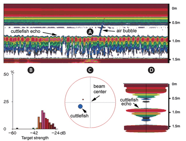
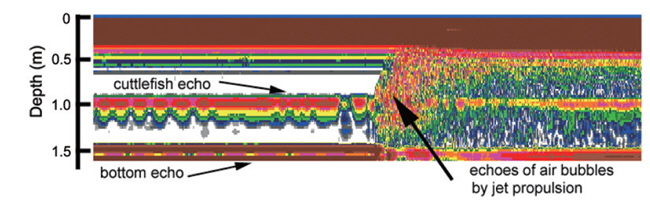
During the experiments, echoes from air bubbles caused by the jet propulsion of the cuttlefish were often observed (e.g., Fig. 8). The air bubbles ascended towards the water surface and transducer faces, and precluded accurate measurements of TS during these periods. The frequent occurrence of this behavior suggests that echoes from bubbles produced by cuttlefish may enhance their acoustic detection, particularly during periods of vertical migrations and feeding. However, the bubble echoes may also degrade the accuracy of acoustic estimates of cuttlefish biomass. More research is also needed to understand the variation in acoustic backscatter from cuttlefish caused by their various behaviors.

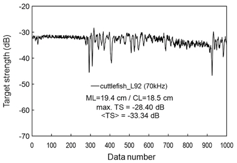
During the experiments, measurements were made of cuttlefish moving quasi-naturally. If the cuttlefish was too active, the measurements were suspended until it was calmed (Huang and Clay, 1980). If the cuttlefish was too calm, it was stimulated. Measurements for a moderately moving cuttlefish are exemplified by an echogram (Fig. 9) and a time series of TS at 70 kHz (Fig. 10). The echoes varied between transmissions due to cyclical contractions of the lateral fins and changes in θ, particularly for the most active cuttlefish. Even for the moderately active cuttlefish, however, the TS measurements ranged approximately 20 dB, from -45 to -25 dB, with a mean equal to -33.34 dB (Fig. 10).

In situ cuttlefish may exhibit behaviors which differ from those observed in these tank experiments. Consequently, their TS values may differ from this set of measurements. Also, not unlike fish with swimbladders (Goolish, 1992; Horne et al., 2000), cuttlefish control their buoyancy (Denton et al., 1961; Denton and Gilpin-Brown, 1961; Denton and Taylor, 1964; Chen et al., 2011) by adjusting the fluid and gas in the many cuttlebone chambers, which likely modulates their TS. Therefore, the effect of the cuttlebone on the TS of cuttlefish must be quantitatively evaluated. This is the subject of another study.