Clouds have a decisive effect on the global climate and hydrological cycle [1]. Small changes in the location (altitude) or frequency of clouds can impact the climate in a very substantial way, and many studies have shown the crucial role of clouds in modulating the climate [2].
Presently, the ground-based instruments used for the measurement of the cloud base height or velocity include radiosonde, cloud radars [3], ceilometers [4], lidars [5], and stereographic cameras [6]. Radiosondes provide accurate cloud base heights, especially for low clouds, but are only released every 12 h or more. Ceilometers, typically as a part of automated airport weather stations, are the most common cloud base height observational tool [7]. In the case of the lidar technique, the light travel length between the transmitter (laser) and clouds is used to measure the height of the cloud base, which is a very accurate and fast method. Furthermore, lidar techniques have many application fields in climate studies. For example, the cloud temperature can be measured using a rotational Raman lidar [8], and lidar backscattering polarization measurements can provide important information on the cloud and aerosol particle properties [9]. Otherwise, it is very circumscribed in cloud velocity measurements because there is no Doppler effect if the clouds move in the perpendicular direction to the laser beam path of Doppler lidar. Therefore, we tried to find a way to measure change of image and to apply it to the lidar technique, which is a powerful technique in the field of climate study. As a result, we have an interest in the digital image correlation (DIC).
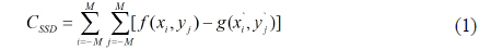
DIC was first developed by a group of researchers at the University of South Carolina in the 1980s when digital image processing and numerical computing were still in their infancy. As a representative non-interferometric optical technique, the DIC method has been widely accepted and commonly used as a powerful and flexible tool for surface deformation measurements in the field of experimental solid mechanics [10]. Among the DIC algorithms, the sum of squared differences (SSD) method is a way to track the sub-set image in different images. We used this algorithm for tracking the same point in different moving cloud images.
In this paper, we propose a new method to measure the cloud base height and velocity. The cloud base height was measured using lidar’s range detection method, and the cloud velocity was measured using the application of the DIC technique for the lidar’s range detection.
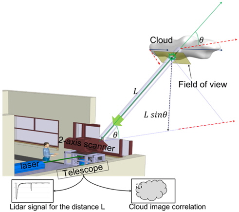
We used lidar signals to measure the distance of L. As shown in Fig. 1, lidar signals show the laser light traveling time from the light source to the clouds. We can acquire the length of L easily by multiplying the traveling time with the light speed. In addition, the height of the cloud can be acquired by using the distance of L and a laser illuminating angle of θ. If the distance is acquired once, we can calculate the actual area of the telescope’s field of view at the position of the cloud. Then the ratio (R=Csize/LCCD) of the imaged cloud pixel size (LCCD) of CCD to the actual size (Csize) of the cloud within the field of view is acquired. Thus, the moving distance of the cloud image in the monitor is converted into the actual moving distance per unit time by the application of this ratio.
We intended to configure the cloud monitoring system as mentioned above, and the following are the configurations of the optical and DIC systems.
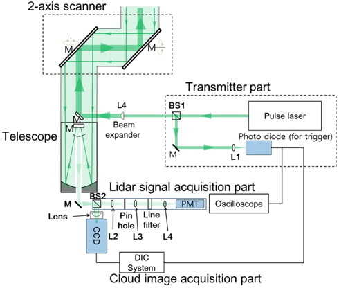
As shown in Fig. 2, our experimental set-up is divided into two major parts. One is the transmitter, which is an injection seeded Nd:YAG laser. The laser beam is split into two paths by a beam splitter (BS1). The transmitted beam passes through the beam expander (L4), and the expanded beam is sent to an elliptical mirror. The beam reflected at the elliptical mirror is sent into the air using a 2-axis scanner with two rotatable mirrors. We use this scanner to find the target cloud and transmit a pulsed laser beam to the clouds. The other is the acquisition part, which is separated into two systems. The scattered laser beam on the target clouds is collected by a telescope and passes through the beam splitter (BS2). The transmitted laser beam is focused on a pinhole by lens (L2). At this time, the pinhole blocks the background signal. After the pinhole, the expanded beam is colliminated by lens (L3) and the colliminated beam is line-filtered by a band pass filter (532 nm). The filtered beam is focused on PMT (Hamamatsu, R9880U) by lens (L4) and the lidar signal is acquired.
[TABLE 1.] Lidar system specifications
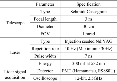
Lidar system specifications
The measurement method using DIC is a vision measurement method, which measures the displacement using a CCD camera and analyzing the correlation of the images before and after the movement. In the measurement method using DIC, the correlations of images taken by a CCD camera before and after a movement are compared to measure the cloud displacement.
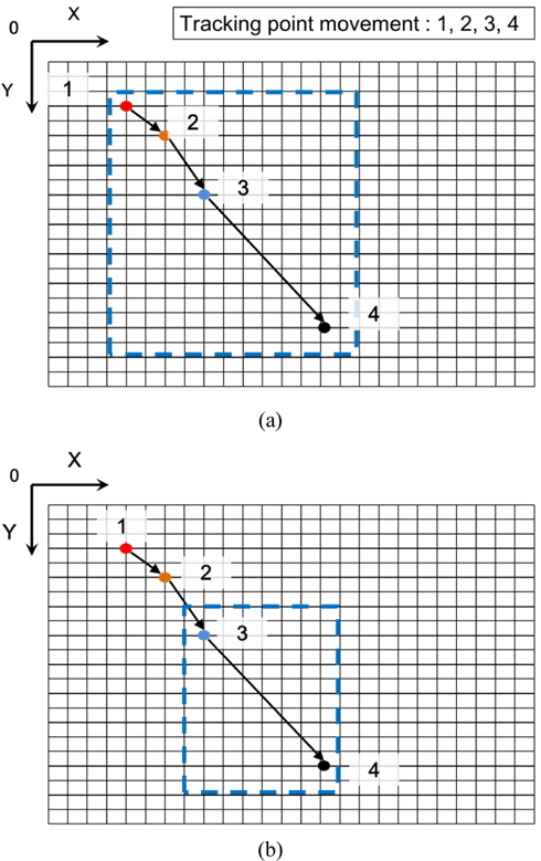
We could not track the cloud image using the conventional DIC algorithm because cloud images change very fast and calculation requirements are huge. We developed a fast correlation algorithm to track the fast moving cloud images. Our fast correlation algorithm is a method to decrease the size of the initial estimation, which is newly set in the next image tracking process. Therefore, the amount of calculations is decreased in the correlation comparison algorithm and the result can be derived quickly. Figure 3(a) shows the size of the initial estimation area for analyzing the cloud displacement, according to the conventional correlation algorithm. As shown in the figure, as the size of the initial estimation area, which includes the largest displacement, increases, the number of repetitive calculations for the correlation comparison is increased. Figure 3(b) shows the initial estimation area for a correlation comparison using the fast correlation algorithm. Here, the coordinates for the correlation comparison of images after movement are applied to the coordinates of the initial estimation area, which are used to analyze the image acquired after movement. Thus, the size of the initial estimation area is decreased and the number of repetitive calculations is decreased.
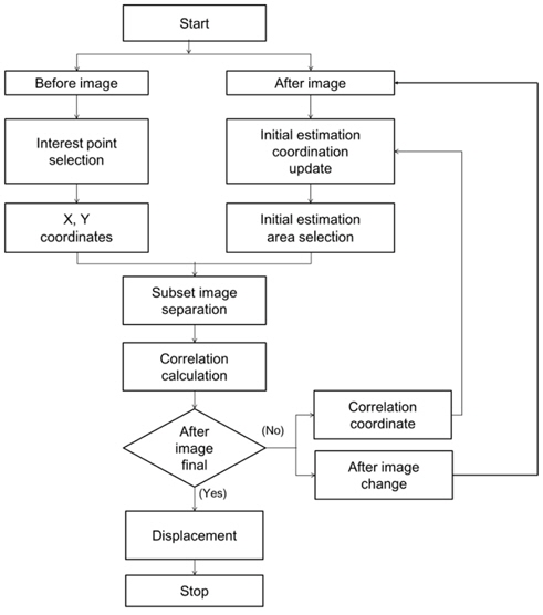
Figure 4 shows the algorithm for a high-speed correlation comparison. The first image (‘Before’ image in Fig. 4) is set up as the reference image among images that the CCD records. We select a point of the reference image to be tracked, then the coordinates of the selected point are set up by algorithm. We separate the subset image from the reference image by unit of (2n+1)ⅹ(2n+1) pixels which is based on the coordinates of the point.
In the second image (‘After’ image in Fig. 4), an initial estimation area is set up which is to be compared and the subset images are separated from the initial estimation area. And then the digital image correlation algorithm calculates the correlation coefficient by using SSD (Sum of Squared Difference) between the subset image of reference and the subset images of the second image. The subset image which has the least value is found among the subset images of the second image and the coordinates of the subset are acquired. We can track the cloud image to record the coordinates of the subset images.
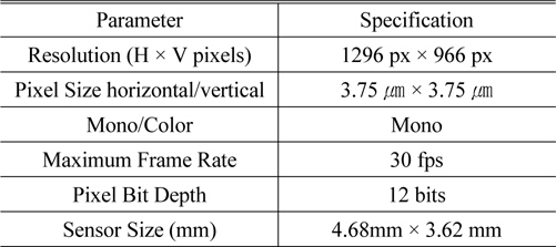
The CCD specifications used are listed in Table 2.

CCD specifications
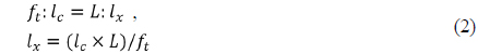
The movements in the cloud images are tracked through pixel coordinate values of the CCD camera. Therefore, to determine the actual movement distance of the clouds, the pixel unit size is converted into the actual distance value. Equation (2) shows the method for determining the distance per pixel to convert the pixel unit value to the actual distance of the movement.

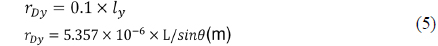
where ft is the focal length of the telescope, lc is the pixel size of the CCD, L is the distance between the telescope and clouds, and lx is the actual length corresponding to one pixel size. Thus, we can acquire the actual moving distance of clouds per unit time along the x-axis using equation (2). When clouds move along the y-axis in the monitor screen, the actual moving distance should be compensated because the light axis of the telescope forms an angle of θ with the direction of the cloud movement. If clouds move with the same height, the following is the compensated equation for the y-axis,

where ly is the actual length corresponding to a one-pixel size.
As we consider the equipment used (the focal length of telescope (ft): 70 mm, the pixel size of CCD (lc): 3.75 um) and the resolution of DIC algorithm (0.1 pixel), the distance resolution of the x and y-direction are equations (4) and (5) respectively.
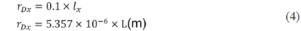


where rDx is the distance resolution of the x-direction, rDy is the distance resolution of the y-direction and rD is the distance resolution of our system.
We used a telescope to acquire the lidar signal and cloud image and found the target cloud by adjusting the 2-axis scanner. The cloud image acquired with the lidar signal was shown in the monitor screen of the DIC system.
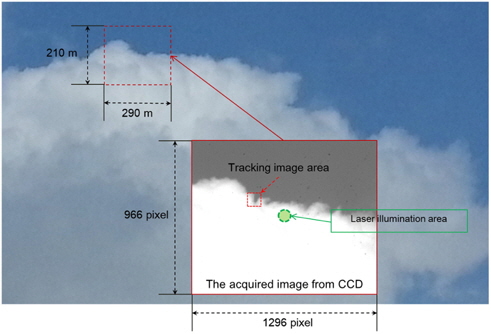
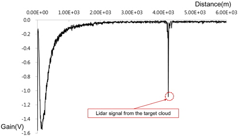
A target cloud image is shown in Fig. 5. The pulse laser illuminated the center of the field of view area of the telescope, and the acquired lidar signal is shown in Fig. 6.
If the tracking cloud images have similar pixel values in the entire area, the DIC algorithm acquires almost the same correlation coefficient at many points in the next image and the DIC system can’t track the images. Therefore, we made our system observe the boundary area of a cloud to adjust 2-axis scanner and set-up the tracking image area in the boundary area.
The scattered laser beam on the target cloud is acquired and that time position is located at about 27.7 μs. Lidar signals were acquired for 10 seconds with a 10 Hz pulsed laser. At this time, the laser illumination angle is 22˚ 1' 7" and the averaged distance to the cloud was 4.15 km for 10 seconds. Therefore, the height of the target cloud can be easily acquired as 1.57 km.
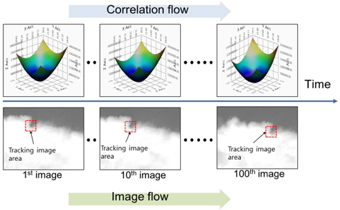
The cloud images were recorded for 10 seconds with a 10 Hz frame rate, and the image tracking process using the DIC system is shown in Fig. 7. The lower figures are cloud images and we can see that the tracking process is held with a high correlation coefficient from the first image to the final image.
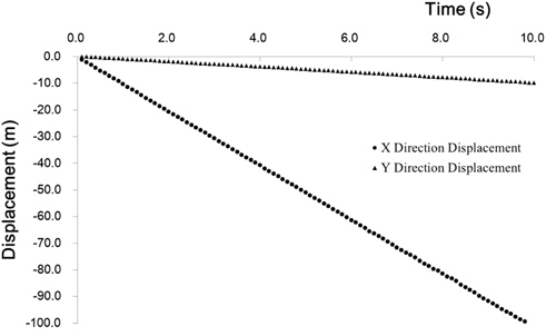
As shown in Fig. 8, the cloud displacements of the pixel unit acquired by DIC are converted into the actual displacements when applying equations (2) and (3), and the velocities of the cloud can be acquired to divide the cloud displacements by the unit time (0.1 second) for the moving directions of x and y, respectively. Finally, the cloud velocities were acquired to sum vectors of the x-axis velocities and y-axis velocities, as shown in Fig. 9.

where v is the cloud velocity,
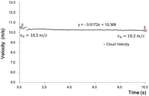
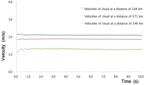
The measurement values of the cloud velocities are shown in Fig. 9. The velocities begin with a value of 10.5 m/s (A point) and decrease slowly. After 10 seconds, the cloud velocity is 10.2 m/s (B point). The measurement values are distributed linearly. Figure 10 shows the results of velocity measurement at the distance of 3.71 km, 3.64 km and 3.46 km respectively.
In this paper, we presented a method for the measurement of the cloud altitude and velocity using lidar’s range detection and the DIC system. For the lidar system, we used an injection-seeded pulsed Nd:YAG laser as the transmitter and a photomultiplier tube (PMT) as the laser light sensor to measure the distance to the target clouds. We used the DIC system to track the cloud image and calculate the actual displacement per unit time. The configured lidar system acquired the lidar signal of clouds at a distance of about 4 km. The developed fast correlation algorithm of the DIC, which is used to track the fast moving cloud relatively, was efficient for measuring the cloud velocity in real time. We acquired the velocities of the cloud at a distance of about 4 km. The measurement values had a linear distribution. If the experimental condition is the same (CCD, distance to cloud, telescope), our system can measure the velocity with a resolution of about 0.1 m/s because our DIC system discriminates one-tenth of the pixel size. If a CCD with a greater number of pixels is applied to the system, the velocity resolution will be more precise. We expect that our method will play a bigger role in observing a cloud state (altitude and velocity) and can be used as auxiliary system for Doppler lidar.