Image skeletonization is a morphological image processing operation that transforms a component of a digital image into a subset, called a ‘skeleton’, of the original component. The skeleton usually emphasizes geometrical and topological properties of the shape. It has been used in several applications, such as computer vision, image analysis, and digital image processing.
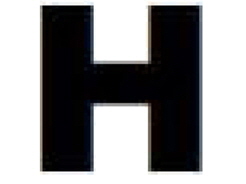
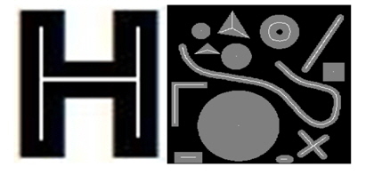
Consider the binary digital character ‘H’ in Fig. 1.
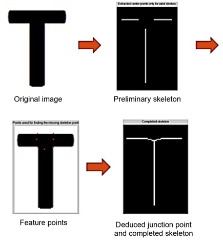
Basically, it consists of three connected strokes (two vertical and one horizontal). The topology, which is the important information for object recognition, represents how the three parts are connected. In such a situation, it will be convenient if the thickness is reduced as much as possible (to a skeleton), so that the topological analysis becomes as simple as possible. For example, it would be nice to represent the pattern above as a one-pixel thick white pattern as illustrated in Fig. 2.
The processes or methods to accomplish this task are called skeletonization or thinning techniques, and the resulting patterns are usually referred to as skeletons.
Nowadays, many graphic and vision applications, which include character recognition, signature verification, and fingerprint recognition, are required to represent and understand the shape of a target object. The skeleton is one kind of shape descriptor [1]. It is a compact, medial structure that lies within a solid object [2]. A skeleton of a 2D object consists of 1D elements (e.g., curve, straight line); whereas the skeleton of a 3D object may consist of both 1D and 2D elements (e.g., surface). A skeleton is a lower dimensional object that essentially represents the shape of its target object. Because a skeleton is simpler than the original object, many operations can be performed more efficiently on the skeleton than on the full object.
Skeletonization is divided into two main approaches: iterative and non-iterative. In the iterative techniques, the peeling contour process is iteratively conducted in a parallel or sequential manner; in the parallel way, the whole unwanted pixels are erased after identifying the whole wanted pixels. Whereas in sequential techniques, the unwanted pixels are removed in identifying the desired pixels in each iteration as in [3]. Examples of pixel-based techniques are thinning and distance transformation. These techniques need to process every pixel in the image; this can incur a long processing time, and leads to reduced efficiency. In the non-iterative approach, the skeleton is directly extracted without individually examining each pixel, but these techniques are difficult to implement and slow [4].
Some thinning methods suffer from common traditional problems, such as the one pixel width of the skeleton and skeleton connectivity. Besides, distortion in the topology of the shape skeleton is a serious problem in thinning applications [5]. Several techniques failed in preserving the topologic shape [6, 7]. Spurious tails and rotating the text shape are other serious problems that most thinning methods failed to solve [6-8].
This paper presents a novel approach based on the stroke width of a target object to extract its skeleton. To the best of our knowledge, this is the first time tensor voting and stroke width have been used in skeletonization.
First, contour from the object is detected by using a Canny edge detector [9] and then tensor voting [10] is applied to estimate the normal vectors of edge pixels in the previous step. Starting from each edge pixel and following its normal vector, its counterpart can be found at the opposite edge. The starting edge pixels and their counterparts form a set of strokes. From these strokes, we have a set of their center points that make up preliminary parts of the skeleton.
Second, we smooth the primary skeletons, and connect them through the junction area, by finding the junction points. The junction points are obtained by an interpolation compensation technique.
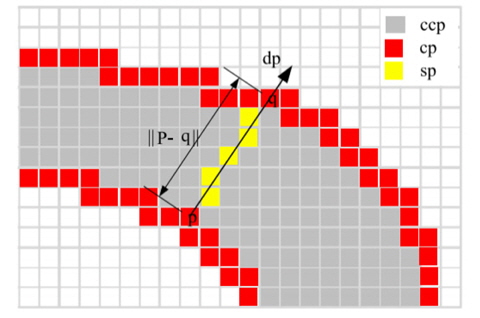
We define a stroke to be a contiguous part of an image that forms a band of nearly constant width as depicted in Fig. 4. We do not assume to know the actual width of the stroke but rather recover it. In Fig. 4, p is a component contour pixel (cp) that lies on the edge. Searching in the direction of the gradient at p leads to finding q, the corresponding pixel on the other side of the stroke. Pixels along the ray form a stroke [11]. These pixels are called stroke width pixels (sp). Candidate component pixels (ccp) lie between the two edges but do not belong to strokes.
>
C. Normal Vectors of Edge Pixels
1) Using Gradient
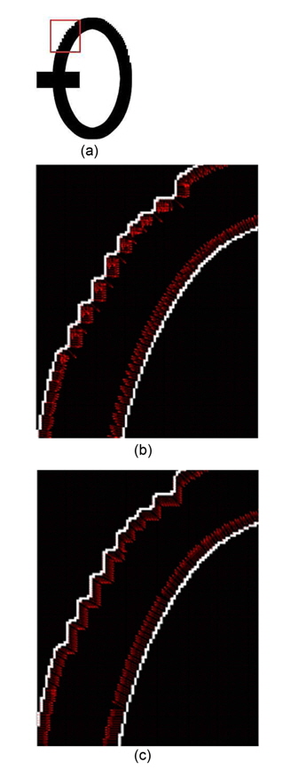
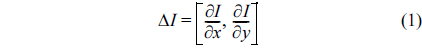
In the gradient method, the normal vector of an edge pixel can be approximated by considering only eight surrounding pixels as in Eq. (1). Therefore, when the edge is not smooth enough, i.e., it has staircase elements, normal vectors would be computed incorrectly. Fig. 5(b) illustrates this situation. In this case, the gradient method is no longer suitable for finding normal vectors. This paper proposes to use a Tensor Voting based method to solve this problem.
where,
2) Using Tensor Voting
The Tensor Voting based method estimates the normal vector based on the pixels in a voting field. Pixels in high-density areas of the voting field contribute more significantly than others.
First, edge pixels are extracted. Coordinates of these edge pixels are input into the Tensor Voting framework [10]. After the voting process, tangent vectors are obtained from the stick tensor. The normal vector is roughly perpendicular to the tangent vector. Fig. 5(c) shows normal vectors that are results from the tensor voting method. In this situation, it is better than the gradient method. Compared to Fig. 5(b), the normal vectors around curves are well computed.
>
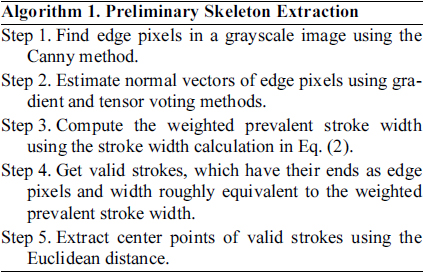
D. Preliminary Skeleton Extraction
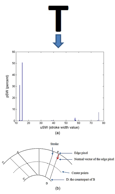
Contour from the object is detected by using Canny edge detector, and then tensor voting is applied to estimate the normal vectors of edge pixels in the previous step. Starting from each edge pixel and following its normal vector, its counterpart can be found at the opposite edge. The starting edge pixels and their counterparts form a set of strokes. Then we have the stroke width distribution. The weighted prevalent stroke width (WPSW) is computed by Eq. (2).

where, uSWi represents one stroke width value in the distribution and pSW is the corresponding percent of that value over the total.
For example, in Fig. 6(a), from the stroke width distribution, we have uSW = {12.64, 13, 13.03, 13.15, 13.34, 14.14, 14.31, 15, 38.27, 39.39, 57, 57, 57.14, 57.21, 57.42, 57.55, 57.70, 75, 76, 76, 76.16, 76.23} and pSW = {0.0043, 0.3013, 0.0087, 0.0043, 0.0043, 0.0043, 0.0043, 0.5065, 0.0043, 0.0043, 0.0131, 0.0043, 0.0262, 0.0087, 0.0043, 0.0043, 0.0043, 0.0043, 0.0698, 0.0043, 0.0043, 0.0043}. By applying Eq. (2), we have WPSW = 22.64; this is the prevalent stroke width throughout the input image.
After that, only strokes that have width roughly equivalent to the weighed prevalent stroke width are kept. From these valid strokes, we have a set of their center points that make up preliminary parts of the skeleton.
Since the proposed method starts from a contour of the object, the existence of edge pixels is crucial for extracting the target skeleton. In the cases of junctions or crossing areas, some edges are missing so that the skeleton cannot be extracted by examining the stroke width alone. The reason is that as the distance between the starting pixel in one edge and its counterpart in another edge (they form a stroke) increase, stroke widths in these areas are considerably larger than the stroke width that is prevalent over the entire image. Strokes in junction areas are discarded because they exceed by far the weighed prevalent stroke width. In this paper, an interpolation compensation technique is used to deal with this problem.
>
E. Interpolation Compensation
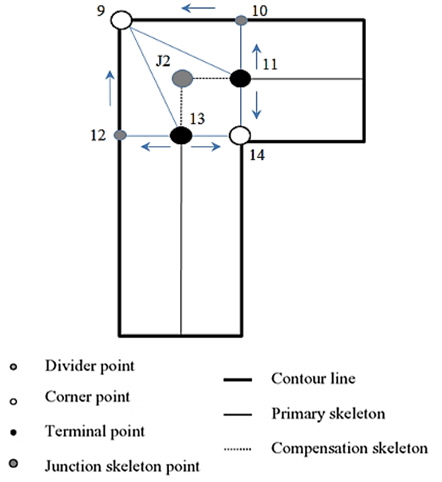
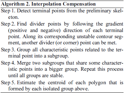
To find junction points that are missing from the preliminary skeleton, we develop an interpolation technique [12]. The key of this technique is to position the junction skeleton points in the crossing area based on three detectable types of characteristic points: terminal point, divider point, and corner point. The junction skeleton point can be estimated in two ways: 1) it is the centroid of the polygon, which is composed of the above three types of characteristic points and 2) the position of the junction skeleton point can be calculated by the least square method with the characteristic points.
The corner points are detected by using Harris corner detection [13] as above. The terminal point is the start or end point of the preliminary skeleton. The divider point is the intersection point between the stable and the unstable contour segments. Along the gradient direction of the terminal point (for example, points 11 and 13 in Fig. 7), the divider points (points 10 and 12 in Fig. 7) can be easily detected. They are illustrated in Fig. 7.
III. EXPERIMENT AND COMPARISON
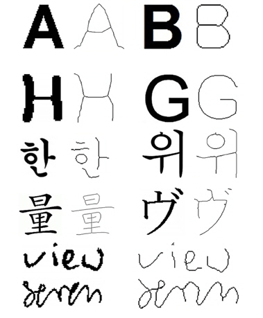
In this section, highlight results of the proposed method are presented and discussed. The algorithm is tested on a variety of inputsisolated letters, handwritten words, and finally, graphics and symbols, regarding skeleton continuity, shape preservation, and a one-pixelwide skeleton. The goal is to verify if the performance complies with the expectations. There are 106 images in the dataset.
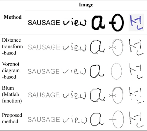
As seen in Fig. 8, the proposed method preserves the letter shapes. It does a good job of maintaining the original connectivity in the output skeletons, which is essential for many applications.
Table 1 shows sample results of the proposed approach in comparison with methods mentioned in the Introduction section.
[Table 1.] Results from the methods discussed

Results from the methods discussed
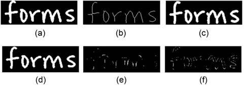
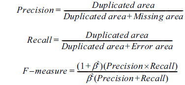
Table 2 presents a comparison between the proposed approach and other methods by quantitative evaluation. The image reconstructed from the skeleton is compared with the original image in terms of duplicated area, missing area, and error area (Fig. 9).
[Table 2.] Comparison with benchmarks
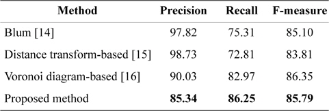
Comparison with benchmarks
● Duplicated area: overlapped parts of reconstructed image (from skeleton) and original image. ● Missing area: parts that exist in the original image, but are missing in the reconstructed image. ● Error area: parts that exist in the reconstructed image, but are missing in the original image.

In our work,
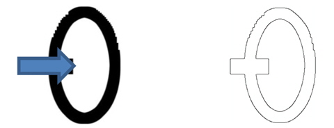
The proposed method has the following strengths: ● It extracts skeletons without spurs or undesirable branches (Fig. 10). ● It is non-iterative and works even when the edge is not smooth enough, i.e., it has staircase elements. ● It is tailored for printed characters, where the stroke width is consistent. ● It is a grayscale skeletonization algorithm that can solve the problem of shape distortion by binarization (as seen in Fig. 11).
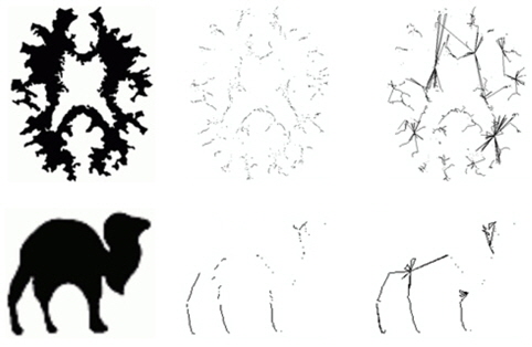
It also has the existing weaknesses (Fig. 12): ● It is a 2D skeletonization method. ● It is sensitive to the stroke width of the target object. ● It fails to produce desirable results in cases of complex shapes.
This paper proposed a novel approach based on the stroke width of a target object to extract its skeleton. First, we detect the contour from the object and use normal vectors, which are estimated by a Tensor Voting based technique to extract strokes between edge pixels. From these strokes, we have a set of their center points that make up preliminary parts of the skeleton. Second, we smooth the primary skeletons and connect them through junction areas by finding the junction points. The junction points are obtained by an interpolation compensation technique. The experimental result proves that tensor voting and stroke width can be used to extract the skeletons of 2D objects. For the purpose of extracting skeletons to reconstruct the original image, the performance of the proposed method can be matched with popular skeletionization methods. In future research, the accuracy for complex shape objects needs to be improved.