With the development of marine science, the underwater acoustic communication technologies are increasingly required in both military and civilian areas [1]. However, the underwater acoustic channel is one of the most complex channels among all communication channels. It is characterized as a multipath induced fading channel due that time variable signal reflections from the sea surface and bottom. There are two sources of time variability: internal changes in the propagation medium such as tide, internal wave and medium time variability, and external changes such as surface fluctuation and the receiver and transmitter change with time [2, 3]. Internal and external changes range relatively on long time scales and short time scales, respectively. Therefore the former do not affect the instantaneous level of a high speed high frequency communication signal (e.g., monthly changes in temperature) even if it affects low frequency communication signal but the latter affect the high frequency communication signal. The short time scale time-varying environmental factors lead to signal amplitude, phase and coherence changing. In addition, the coherence bandwidth and fading feature also vary over time, which can cause inter-symbol interference (ISI) [4, 5].

There have been many studies for underwater acoustic communication technologies such as modulator, equalizer and encoder[6, 7]. However, there are only a few studies for effects of environmental factors such as effect of thermocline on non-coherent frequency shift keying (FSK) modulation [8].

In this paper, how QPSK performance is affected by sea surface time variation, was examined in two different sea surface conditions.

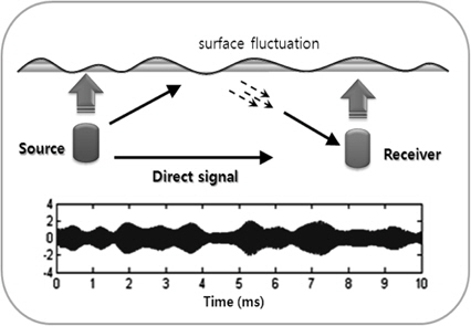
Fig. 1 is adopted from our previous underwater acoustic channel simulation work and it shows signal fading principle due to interference of direct and surface scattered paths [9]. The fluctuation surface produces upper and lower side bands in the spectrum of the reflected sound that the duplicates of the spectrum of the surface motion.

As shown in Fig. 1, the signal fluctuates in amplitude and phase. In this case, the equivalent low-pass received signal r_l(t) is given as [9]

Where α, β(t), Φ(t), s_l(t) and z(t) are the amplitude of the direct path signal, attenuation factor of surface reflection path, phase change of surface reflection path, transmitting signal and uncorrelated noise, respectively. In eq. (1), the time-variant complex envelopes of α + β(t)e^-iΦ(t) depend on the direct path amplitude and the attenuation factor of surface reflection and 2^nd term in eq.(1) is controlled by the surface roughness parameter or the Rayleigh parameter. The Rayleigh parameter is defined as R = khsingθ, where k is the wave number, h is the effective value of the surface wave height, and θ is the grazing angle. When R ≫1, the surface acts as a scatter, and the scattering path reflected from a surface wavelet will have a sea surface wave fluctuation frequency. Then the envelopes |β(t)e^-iΦ(t)| and |α + β(t)e^-iΦ(t)| are Rayleigh distributed and Rice distributed, respectively.

Equation (1) is characterized by the channel coherence bandwidth B_c (inverse of time spread T_c) and the coherence time T_d (inverse of Doppler spread B_d) and the former and the latter control the signal bandwidth and the signaling interval, respectively.

The time spread T_c in the discrete multipath channel is evaluated as

Here, the average delay and are given as

Here, P(_𝜏k) is the intensity of the k^th path.

Temporal coherence time T_d is defined by the correlation of the signals separated by a delay time 𝜏, normalized by the power of the signal, as given by

Where [p^*(t)⊗p(t + 𝜏)] means the maximum value of the cross-correlation of the two time series or the convolution of the time-reversed signal (denoted by *) with the other signal [10].

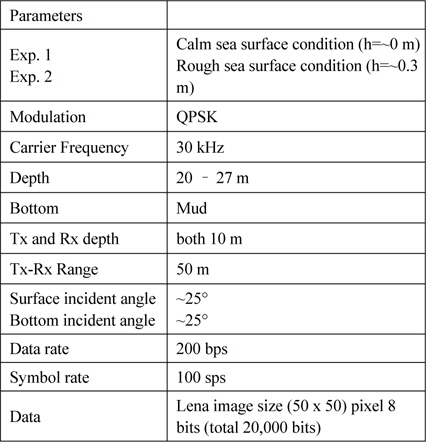
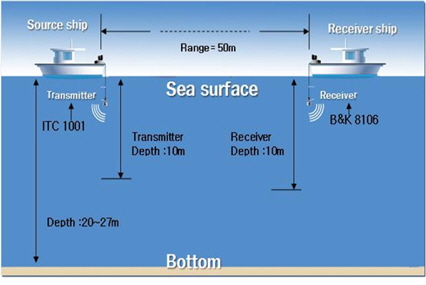
The experiment was conducted in about 20m depth beach near Geoje island in Korea on March 29, 2013. The experimental configuration and parameters are shown in Fig.2 and Table 1, respectively.

The range between the transmitter and receiver is set to be 50 m and the depth of receiver and transmitter are set to be both 10 m. Data rate is 200 bps, so Lena image data that the total number of which is 20,000 bits is divided into 200 frames.

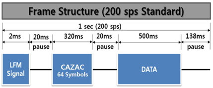
Fig.3 shows frame structure of transmitting signal. Transmission time of one frame is 1 s. LFM ping and CAZAC code signals have good correlation properties. LFM signal was used for the purpose of measuring the channel time spread and the temporal coherence. The minimum and maximum frequencies of LFM signal are set to be 25 and 35 kHz which is greater than signal bandwidth. CAZAC 64 symbol codes were used for frame synchronization. The experiment was conducted in the morning with calm sea surface condition (Exp. 1) and in the afternoon with relatively windy rough sea surface condition (Exp. 2). Even the transmitter and receiver are tethered together the range between both was changed by test ships moving by wind force.

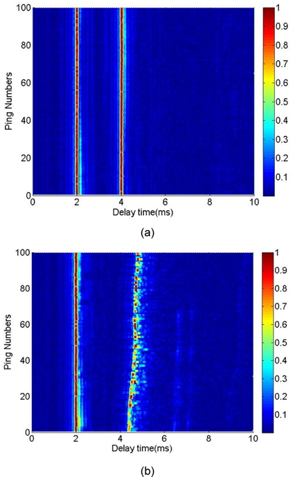
The channel responses by matched filtering the received and the transmitted LFM signals are plotted in Fig.4 displaying the multipath arrivals which only contain directed and sea surface reflected signals as a function of delay time and ping numbers. Bottom reflected signal was not found. As shown in Fig.4, the direct signal intensity and delay time of each ping are pretty stable in both Exp. 1 and Exp. 2 but those of surface reflected signal in Exp. 2 are unstable.

By eq. (2) and (3), the time spread T_c is analyzed to be less than about 1 ms in both Exp. 1 and 2. Therefore the channel coherence bandwidth is approximated to be 1000 Hz.

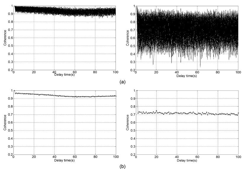
The LFM signals were also used to estimate the temporal coherence T_d. Take one LFM signal as the reference signal and correlated with the signals arriving at a later time. The maximum values of the correlations are entered in Eq. (4) and one obtains one temporal coherence curve. Take a different LFM signal as the reference then one obtains a distribution of temporal coherence curves at different ping number or geotime.

Fig. 5(a) shows the distribution of temporal coherence of LFM signals at different geotimes for Exp. 1 and 2. Fig. 5(b) shows the average of all corresponding temporal coherence distribution. As shown in Fig.5, the average coherence of Exp. 1 is greater than about 0.9 and therefore the coherence time is considered to be long. However, the coherence of Exp. 2 drops to 0.7 after delay time of 1 s and the coherence time is less than 1 s. Here, the coherence of 0.9 is used for criteria of coherence time decision. It is interpreted from this result that the sea surface scattering and range variation between the transmitter and receiver affect the communication performance. The spread factor which controls the signal bandwidth and signaling interval of fading channel is defined as T_c divided by T_d. The spread factors of Exp. 1 and 2 are about 0 and 10^-3, respectively. Since signal bandwidth of 100 sps QPSK is 50 Hz and less than the channel coherence bandwidth of 1000 Hz, the channel is frequency-nonselective. In addition, the channel is slowly fading since T_d of 1 s is greater than the signal interval of 10 ms.

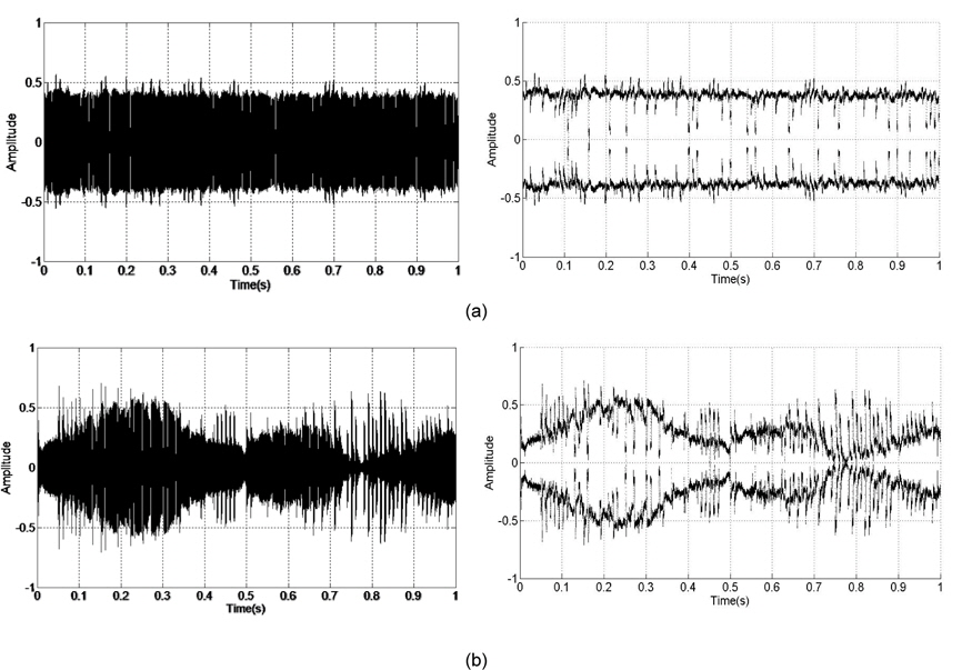
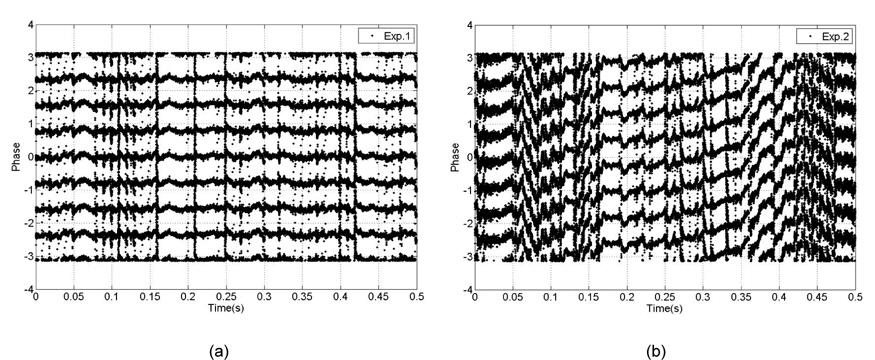
Fig.6 shows the 1 s received signals and the envelopes for Exp. 1 and 2. Fig. 7 shows the time variations of the phases measured at 9 sampling points in each one carrier frequency interval. As shown in Fig. 6 and 7, amplitudes and phases of received signals were changed with time especially in Exp. 2. The surface reflected signal amplitude and phase change with time and fading is induced as clearly shown in Fig. 6(b) and 7(b). The amplitude change may follow the surface wave fluctuation and is caused by time variant interference of the direct and the surface reflected path signals. Considering eq. (1), the envelope of the amplitude will have Rice distribution. The phase variation of Exp. 1 is stable with constant mean value but that of Exp. 2 is unstable with a different mean value with time. Therefore the carrier phase estimation is more important in demodulation process.

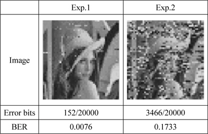
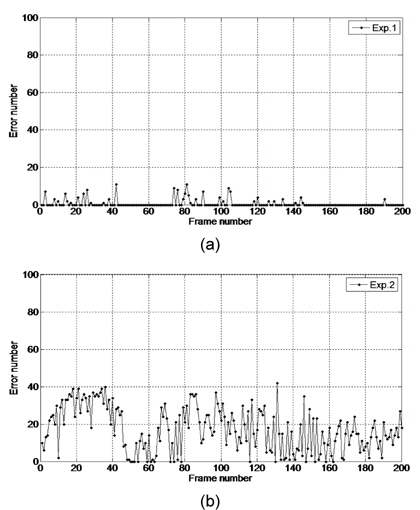
Table 2 shows the received images and the bit error rates (BERs) of Exp. 1 and 2. Here, the received signal was demodulated without the carrier phase estimation. As shown in Table 2, the image quality of Exp. 2 is much worse than that of Exp. 1. The BERs of Exp.1 and 2 are 0.0076 and 0.1733, respectively. Fig. 8 shows the error number to each frame which has 100 QPSK symbols. These results show that the surface scattering due to surface fluctuation controls the performance of QPSK. The system performance of Exp. 2 is worse than that of Exp. 1. Both channels of Exp. 1 and 2 are frequency-nonselective slowly fading, but the amplitude and the phase variation of frame by frame of Exp. 2 give worse performance than Exp. 1. Therefore, the quality of signal greatly depends on the time variation of environmental factors of communication channel. Another finding is that the error number variation of each frame is not uniform in Exp. 2. This is also explained by time variation of amplitude and phase which is controlled by time variation of sea surface scattering. So a good demodulation method with the carrier phase estimation is very critical in the future QPSK system design.

Performance of QPSK system is examined through the image transmission in the calm and the rough sea surface conditions. Fading feature induced by a direct and a surface scattering is analyzed. The time spread and the time coherence are analyzed using LFM ping signal and the channel is found to be frequencynonselective slowly fading. The received signal of QPSK shows the time variable amplitude and phase especially in the rough sea surface condition. The amplitude and phase of the received signal are closely related to time variation of sea surface fluctuation. By relating these with time variant envelope, amplitude and phase of received signal, it was found that the bit error rates (BERs) of QPSK are closely related to time variation of sea surface state.