The occurrence of unsteady cavitation in pump is nearly inevitable, where the local pressure drops below the saturated vapor pressure, especially for those applied on vessels and offshore platforms, since the particles contained in seawater can increase the probability of cavitation generation. Cavitation may cause various problems, like vibration, noise and material erosion, which would deteriorate the pump performance and cause damage to the pump (Brennen et al., 1995; Ding et al., 2011; Bruno and Frank, 2009). In the recent years, owing to the continuous improvement of Computational Fluid Dynamics (CFD) technologies and computational capabilities, the prediction of pump cavitation performance based on CFD method has been beneficial for preliminary pump design (Liu et al., 2010; 2012; Wang et al., 2011; Dijkers et al., 2005). Thus, it makes the cavitation model play a significant role in numerical simulation progress. During the last decades, great efforts have been made in the development of cavitation models (Athavale et al., 2002; Coutier-Delgosha et al., 2003). These models can be put into two categories, namely interface tracking methods (Senocak and Shyy, 2004; Hirschi et al., 1998) and homogeneous equilibrium flow models (Zwart et al., 2004; Kunz et al., 2000; Singhal et al., 2002; Schnerr and Sauer, 2001; Merkle et al., 1998; Delannoy and Kueny, 1990). The former assumes that the cavity region has a constant pressure equal to the vapor pressure of the corresponding liquid and the computations are calculated only for the liquid phase. However, these methods are limited to 2-D planar or axisymmetric flows because of the difficulties dealing with complicated 3-D models. In the second category, the homogeneous equilibrium flow models assume the flow to be homogenous and isothermal, applying either a barotropic equation of state or a transport equation for both phases. The barotropic equation links the density to the local static pressure (Delannoy and Kueny, 1990). A recent experimental study implied that the vorticity production is an important aspect of cavitating flows, especially in the cavity closure region (Gopalan and Katz, 2000). But in the barotropic law, the gradients of density and pressure are always parallel, which leads to zero baroclinic torque. Therefore, the barotropic cavitation models cannot capture the dynamics of cavitating flows, particularly for cases with unsteady cavitation flows (Senocak and Shyy, 2002). Furthermore, this method is prone to instability because of high pressure-density dependence, which makes it difficult to reach the convergence levels of noncavitating flow simulations (Marina, 2008). Conversely, these limitations can be avoided by applying the transport equation models (TEM). In this approach, volume or mass fraction of the two phases are solved by an additional transport equation with different source terms. Besides, there is another apparent advantage of this method, which could predict the impact of inertial forces on cavities like elongation, detachment and drift of bubbles. In the past years, a great number of transport equation models are proposed (Zwart et al., 2004; Kunz et al., 2000; Singhal et al., 2002; Schnerr and Sauer, 2001; Merkle et al., 1998). These models apply different condensation and evaporation empirical coefficients to regulate the mass and momentum exchange. However, most of these empirical coefficients are calibrated on simple hydraulic machinery, such as hydrofoil or blunt body. When these models are employed in pumps, the accuracy of numerical simulation is strongly dependent on users’ experience to choose proper coefficients. Among this kind of TEM models, because of its effectively and stability, the Zwart-Gerber-Belamri model (hereafter ZGB model) was widely used for different cases (Zwart et al., 2004; Hagar et al., 2012; Liu et al., 2012).

In this study, the influence of the empirical coefficients on predicting the cavitation performance of a centrifugal pump was investigated. To this aim, the ZGB model was considered. Moreover, the experiments were carried out to validate the numerical simulations.

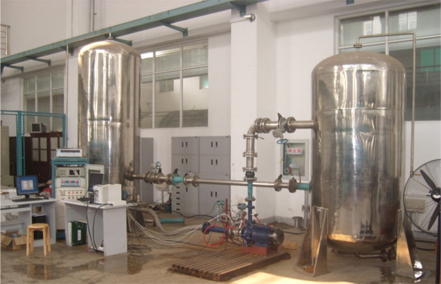
The experiments were performed on a closed platform in the Research Center of Fluid Machinery Engineering and Technical of Jiangsu University. Fig. 1 shows the centrifugal pump closed test rig. Two pressure transducers, JYB-KO-HAGL- 1, are installed in the upper and down steam, with a measurement accuracy of ±0.5％FS (The FS is interpreted as the full scale of the pressure transducer, which is ±100kPa). To avoid the disturbance from the pump, a turbine flowmeter LWGY-80A is mounted far away from the pump, with an accuracy of ±0.5％ for the flow-rate value between 16-100m³/h. Measurement uncertainties were estimated to be less than ±2％ and ±1.5％ respectively, contributing to an uncertainty of ±2.8％ of the pump head and ±2％ of the cavitation number, according to Eqs. (9) and (11). All of the measured data are acquisitioned synchronously and then processed by a pump test system, TPA, developed by our research center. The ambient temperature is about 22° and after 3 times tests, the system is ceased for hours until the water temperature cools down.

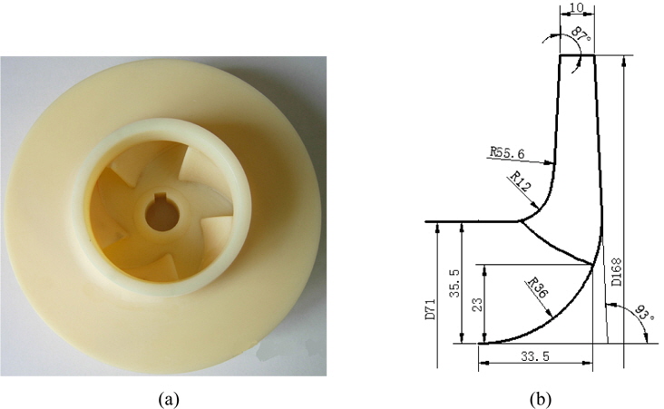
The basic parameters of the test pump are listed as follows: the volume flow rate Q = 0.014m³/s, the rotation speed n = 2,900r/min, the impeller diameter D₂ = 168㎜ and the blade number Z = 5. The impeller test model is given in Fig. 2(a), which is manufactured by the rapid prototyping technology. Its meridional shape is also plotted in Fig. 2(b).

The set of governing equation consists of the mass continuity (1) and momentum Eq. (2) plus a transport Eq. (3) to define vapor generation:

The mixture density is defined by the vapor volume fraction, expressed as:

where p is the pressure, ρ_m is the mixture density, u_i is the velocity, μ and μ_t stand for the laminar viscosity and turbulent viscosity, α is the volume fraction, and represent the source terms for evaporation and condensation. The subscripts m, l, v indicate the mixture, liquid and vapor, respectively.

The RNG k-ε model was adopted for solving the transport equations of the turbulent kinetic energy and its dissipation rate, which is based on the renormalization group analysis of the Navier-Stokes equations. The RNG k-ε model has been proved to give good predictions in cavitating flows (Zhou and Wang, 2008; Chang and Wang, 2012; Yang et al., 2012). To improve the numerical simulations, a modification of the turbulent viscosity was taken into account to reduce the turbulent viscosity of the mixture, proposed by Coutier-Delgosha et al., (2003). The turbulent viscosity μ_t is defined as

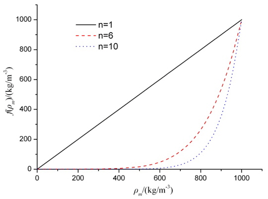
where the exponent n is a constant and Fig. 3 shows the relationship between different n values with f(ρ_m). It can be noted that, with increasing n, the turbulence viscosity would reduce obviously. As recommended by Coutier-Delgosha et al., (2003), n = 10 was employed in the present study.

All the simulations were conducted by using the ANSYS-CFX commercial software and the ZGB model was considered in this paper, which is deduced from the Rayleigh-Plesset equation:

where F_vap and F_cond are the empirical calibration coefficients of evaporation and condensation, respectively. And r_nuc is the nucleation site volume fraction, R_B stands for the nucleation site radius (hereafter NSR). Vaporization is initiated at nucleation sites, which can be regarding as the non-condensible gases. p_v represents the water vaporization pressure. The recommended values of these coefficients are: F_vap = 50, F_cond = 0.01, r_nuc = 5 × 10⁻⁴, R_B = 2 × 10⁻⁶m and p_v = 3574Pa. In this paper, the coefficients, F_vap, F_cond and R_B, were studied to find out the influence on predicting the cavitating flows in centrifugal pump.

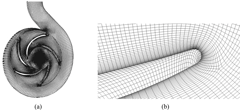
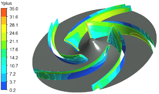
To get a good accuracy computing results, the structured hexahedral grids were generated by GridPro commercial software. Fig. 4(a) shows the computational fluid domain of the centrifugal pump. The grids near the blade surface region layer were refined, which is locally zoomed up in Fig. 4(b). The Y plus on the blade surface is ranged from 0.2 to 35 (Fig. 5). To get a relatively stable upper and down stream flow, two prolongations, whose lengths are four times of the pipe diameter, were assembled on the impeller and volute.

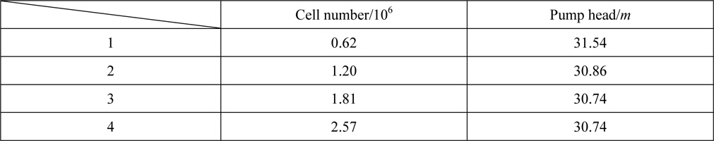
A mesh independence test was performed based on the pump head H under non-cavitation condition, calculated by Eq. (9).

where p_tin and Pp_tout represent the total pressure of the inlet and outlet, respectively.

Table 1 gives the simulation results with five different kinds of grid density. It is obviously that when the cell number is over two million, the discrepancy of the pump head is within 1％. Ultimately, considering the simulation efficiency, the total cell number of all the domains are set as 1.20×10⁶.

In the simulation process, since the pump impeller is a rotating part, whereas the other parts, the prolongations and volute casing, are stators, the Multiple Reference Frame (MRF) approach was employed, which allows the analysis of situations involving rotator/stator fluid domains and has been demonstrated that it has good accuracy (Ding et al., 2011; Tan et al., 2012). The interfaces were imposed between the impeller and inlet prolongation and volute. The pressure and mass flow rate boundary conditions were fixed at the inlet and outlet, respectively. Moreover, no slip boundary condition was applied on the solid surface of the pump. All the calculations were firstly carried out under non-cavitation condition to obtain a steady solution. Then, the pressure loaded on the inlet was decreased progressively until the desired cavitation number was reached.

In the convenience of comparing the results, two dimensionless parameters are defined as:

where u₂ is the circumferential velocity at the impeller outlet, p_in represents the static pressure of the inlet.

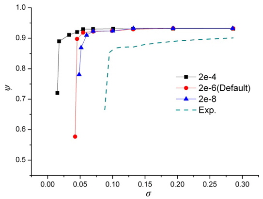
In Fig. 6, the pump head drop characteristic curves are shown, calculated by different NSR, while the other empirical coefficients are set as default. To distinguish the experimental results from the numerical simulations, the experimental results are plotted as dash line, whereas the straight lines with symbols stand for the computed results. Apparently, the smaller NSR, such as R_B = 2 × 10⁻⁸m, the closer the results to the experiment. Under non-cavitation conditions, compared with the experiment, a slight overestimation of the pump head can be observed in simulations. Here we define a scaleless parameter-the critical cavitation number σ_c as the σ value when the pump head drops by 3％. The σ_c values of each conditions are 0.027, 0.048 and 0.059, successively from R_B = 2 × 10⁻⁴m to 2 × 10⁻⁸m, whereas the value in the experiment is 0.138, almost three times larger than R_B = 2 × 10⁻⁶m (default).

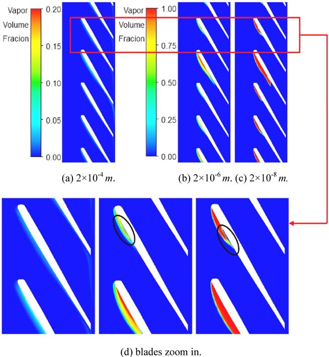
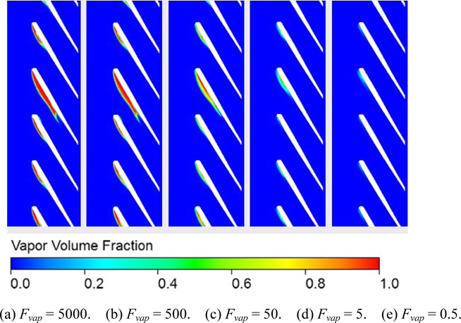
In Fig. 7, the vapor volume fraction distribution with various R_B when σ = 0.07 at Span = 0.5 are plotted. The Span is defined as the dimensionless distance (0-1) from the hub to shroud. It’s important to note the rotating direction is from bottom to top and the flow direction is from left to right. As seen, great discrepancy can be observed. When R_B = 2 × 10⁻⁶m, the cavity region, where the vapor volume fraction is nearly 1.0, is attached on the suction side of the blade surface, and then the fraction gradually decreases in the normal direction. However, as R_B rising to 2 × 10⁻⁴m, there are only a few bubbles with very low volume fraction (Notice that the legends are different from the others). In the opposite case, when R_B reduces to 2 × 10⁻⁸m, the cavity region is approximately identical with the case of R_B = 2 × 10⁻⁶m, except for the high vapor volume fraction area. In the case of R_B = 2 × 10⁻⁸m, the cavity region with high fraction is much larger than the others, contributing to producing a larger low pressure region on the blade surface. This can be observed in Fig. 8, which presents the blade loading distribution on the middle streamline at Span = 0.5 when σ = 0.07. The horizontal axis, streamwise, stands for a streamwise coordinate that follows the blade surface and it ranges from 0 at the leading edge to 1 at the trailing edge of the blade. The vertical axis represents the pressure loading on the blade surface. All the data are computed from the blades zoomed up in Fig. 7(d).

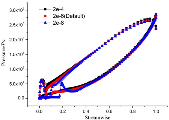
In Fig. 8, the upper curves are the data of the pressure side, while the below ones are the suction side. We can find that the pressure loading distributions on both sides of the blade are almost similar under different NSR, except for the leading edge of the suction side. For the case of higher NSR, the pressure on the suction side gradually rises from the leading edge to the trailing edge. It is mainly because there are a few bubbles with low volume fraction attached on the blade surface (Fig. 7(d)). The situation becomes different when the NSR drops. Due to the bubbles with high vapor volume fraction attached on the leading edge of the suction side, the pressure on this place are approximately zero and the length of the low pressure region increases with the decreasing NSR. For R_B = 2 × 10⁻⁸m, the length is around 0.18, compared with the case of R_B = 2 × 10⁻⁶m, whose low pressure region length is about 0.1. Meanwhile, it is interesting to see that the pressure gets a sharply increase just after the low pressure region and then it has a slightly decline, which is much more obvious when RB = 2 × 10⁻⁸m. The reason lies in the fact that the re-entrant jet in the cavity region near the blade surface, keeps the bubbles away from the blade, which is emphasized in Fig. 7(d) by black ellipses. And as the detached cavity gets close to the blade surface, the pressure drops a little bit and then soars again. Besides, on the pressures side of the leading edge, a humped curve is also observed of all the cases, which is probably caused by the high curvature, leading to flow separation at that point.

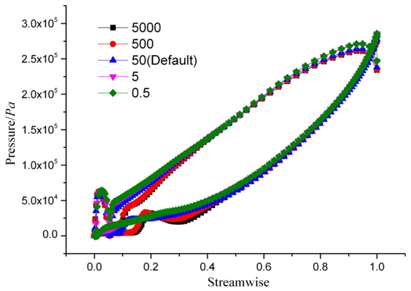
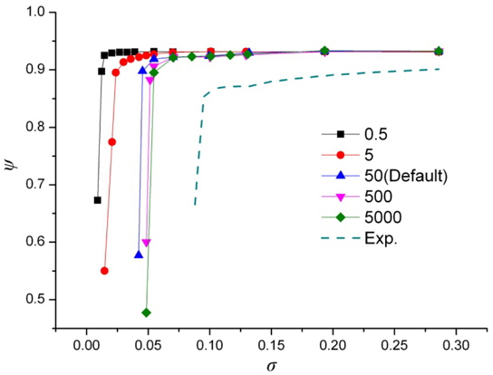
Since the evaporation and condensation coefficients have much more influence on the calculation, more schemes are chosen. The results are given in Fig. 9. As seeing, the smaller F_vap value, the greater discrepancy between the numerical simulation and the experiment. It can be observed that when F_vap＜50(default value), the pump head starts to drop at a very low cavitation number. For F_vap = 5, the critical cavitation number σ_c = 0.027 and for F_vap = 0.5, this value drops to 0.013. It is implied that reducing the F_vap value would greatly impact the computed result. In contrast, when increasing the evaporation coefficient, a slightly improvement of the head drop curve can be noticed. But compared with the experiment result, σ_c = 0.138, the critical cavitation number only goes up to 0.054 and 0.06, respectively for F_vap = 500 and F_vap = 5000.

Figs. 10 and 11 present the vapor volume fraction distribution and blade loading distribution with various evaporation coefficients under the same conditions as Figs. 7 and 8. From Fig. 10, it can be find out that both of the cavity size and length are getting smaller and shorter as the evaporation coefficients declining, leading to diminishing the low blade loading region, as can be seen in Fig. 11. In addition, it is obviously that when the F_vap value increases, the cavity region with high vapor volume fraction become larger.

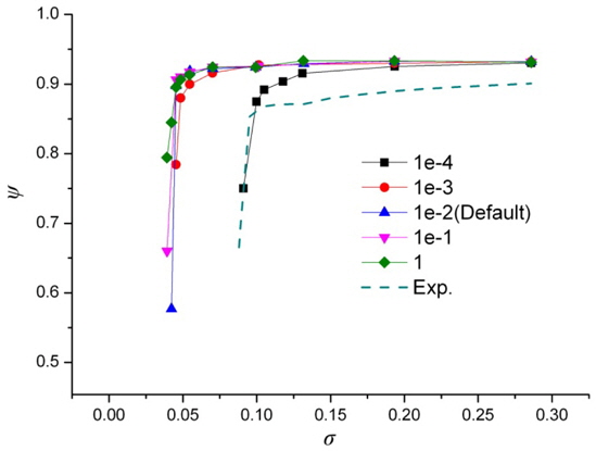
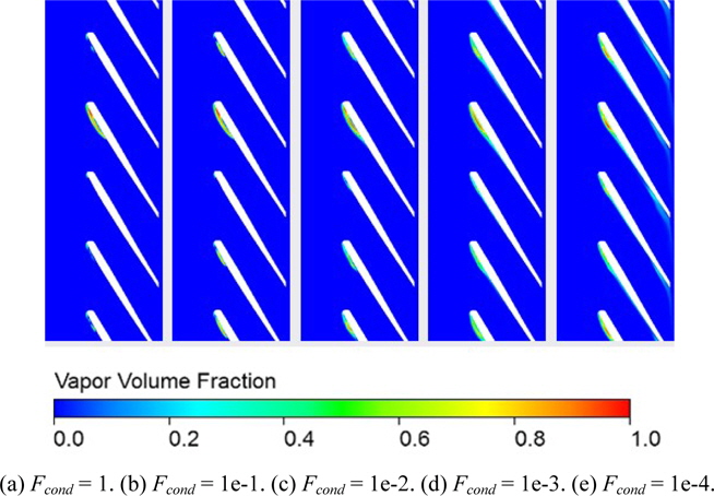
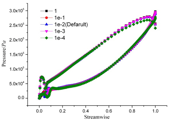
Fig. 12 shows the head drop curves with different condensation coefficients. Similarly, five values are selected to investigate. We can see when increasing F_cond from 1e-2 to 1e-1 and 1, the head drop curve nearly has no change. The critical cavitation number σ_c are 0.047 and 0.045, respectively for F_cond = 1e-1 and 1, compared with σ_c = 0.048 as F_cond = 1e-2 (default value). While F_cond drops to 1e-3, a better prediction result is obtained. The pump head starts to decline when σ is around 0.07, contributing to a higher critical cavitation number σ_c = 0.059. But when the condensation coefficient F_cond reduces to 1e-4, a tremendous improvement can be noticed in the figure. The head drop curve has a good agreement the experiment, with a critical number σ_c of 0.116, compared with 0.138 in the experiment.

Since the cavitation number in the case of F_cond = 1e-4 is higher than the others, the operating condition of σ = 0.1 is chosen to study the vapor volume fraction distribution, which is shown in Fig. 13. It is noticed that with the condensation coefficient dropping, the cavity length is getting longer. As F_cond = 1e-4, the bubbles nearly cover all over the suction side of the blade, which produces a more accuracy prediction results. The reason lies in that, with lower condensation coefficient, the mass of vapor transferred into liquid decreased, making the cavity length much longer. Furthermore, we can find that the cavity of high volume fraction is almost unchanged with decreasing F_cond. Also, the blade loading with various condensation coefficients are plotted in Fig. 14. No remarkable difference can be observed, that is to say, the most affective factor for blade loading is the cavity region of high volume fraction, but not the cavity length.

To investigate the influence of the empirical coefficients of cavitation model on predicting cavitating flow in centrifugal pump, numerical simulation and experiment are presented in this paper. The widely used Zwart-Gerber-Belamri cavitation model is considered. Within this model, three coefficients are analyzed, namely the nucleation site radius R_B, evaporation and condensation coefficients, F_vap and F_cond. During the simulation process, when one of these coefficients is studied, the others are set as default. The conclusions could be arrived at as follows:

(1) The nucleation site radius is considered in the first place with three different values, RB=2×10−4m, 2×10−6m and 2×10−8m. Compared with the experiment, the computed results show that the accuracy of the predictions of the pump cavitation performance is improved as the NSR decreasing. Meanwhile, the vapor volume fraction distribution and the blade loading distribution under certain operation condition are analyzed. For smaller NSR, both of the cavity length and the cavity region of high volume fraction increase, which would promote to degrade the pump head. Besides, because of the re-entrant jet, the low pressure region on the leading edge of the suction side of the blade is much larger with small NSR. (2) Then, the evaporation and condensation coefficients are researched. It can be noticed that, to obtain more precisely simulation results, one can either increases the evaporation coefficient or decreases the condensation coefficient. Moreover, it is important to note that the later approach has much more impact on the predictions than the former and produces progressively better results. To figure it out, the vapor volume fraction distribution is also studied. It is concluded that, the evaporation coefficient controls both the cavity length and the high vapor volume fraction cavity region, and the later factor is more affective on the pressure loading on the blade, but less effective on numerical predictions. On the other hand, the condensation coefficient mostly regulates the cavity length, while the high vapor volume fraction nearly remains identical. And it is observed that, when the cavity covers all over the suction side of the blade, the simulation result has the best agreement with the experiment. However, while the cavity length is within the blade, the simulation results have only a little change. Hence, comparing the influence of the evaporation and condensation coefficients, we may draw the conclusion that the cavity length is the most effect factor degrading the pump head. While the cavity region with high vapor volume fraction is the main factor which impacts the blade loading pressure greatly, but has little impact on the improvement of numerical predictions.