There has been increasing research into the development of unmanned vehicle systems (UVS) that will help save human labor or even human lives in dangerous environments. A successful UVS must feature several technologies, including localization, path planning, and control, if it is to be autonomous [1-4].
Typically, in unmanned aerial vehicle (UAV) systems, autonomous navigation plays an important role in gathering information from the ground [5]. Particularly for military operations in dangerous zones, UAVs undertake a variety of valuable missions such as surveillance, monitoring, and even defense. Most military UAVs adopt a conventional take-off and landing design that requires a long range and a wide and long runway to take off and land.
However, surveillance in complex environments such as urban areas requires a different take-off and landing approach. UAVs need to be capable of vertical take-off and landing in a limited space [6, 7].
Recently, the use of fan-type power has attracted the attention of researchers developing small UAVs for taking off and landing in confined areas. Instead of using a single propeller, four equal-sized fans are utilized. Since such a “quad-rotor” system has four equal-sized fans, it can generate a greater amount of thrust and thus realize more stable hovering control.
Although quad-rotor systems are affected by wind and suffer from limited battery capacity when operating in an outdoor environment, these systems have attracted researcher’s attention owing to their apparent suitability for performing certain tasks. Such tasks include traffic monitoring on highways and the surveillance of accidents on the road.
Considerable research has been undertaken into the development of quad-rotor systems. Quad-rotor systems have already been applied to surveillance tasks [8-18], and aggressive maneuvering control has also been implemented [19]. Excellent maneuvering control has been demonstrated for small quadrotors developed at the University of Pennsylvania. While most quad-rotor systems focus on flying, Flymobile focuses on both flying and driving, and we have performed successful flying and driving tests [20, 21]. Recent research into quad-rotor systems has focused more on localization based on sensors [22-24].
In this study, a novel design was developed for small quadrotor systems meant for private use such as control education or hobbies involving radio-controlled systems, with the goal of producing a smaller, cost-effective unit. Another reason for downsizing the system was to improve the maneuverability of the quad-rotor system. Its small size allows high speed and rapid changes in direction to increase its mobility.
Since the quad-rotor system is small, there are several practical limitations affecting the implementation of the system at a price point that is affordable for public use. However, the reduction of cost involves several technical constraints:
1) The structural size is reduced to attain better maneuverability. The mass is less than 1 kg, and the length is 0.5 m. 2) The control hardware is limited to an 8-bit processor such as an AVR, rather than a digital signal processor (DSP) chip. Some mathematical functions such as square root and arctangent must be approximated since they are beyond the capabilities of 8-bit processors. 3) Algorithms related to the control and sensing processes must be shortened in order to minimize the calculation time in line with the sampling time for practical control. 4) Integer-based operations are required for numerical calculations.
After compensating for the aforementioned problems, we actually implemented a small quad-rotor system. Experimental studies of several flying tests in both indoor and outdoor environments were conducted to demonstrate the operational abilities of the system.
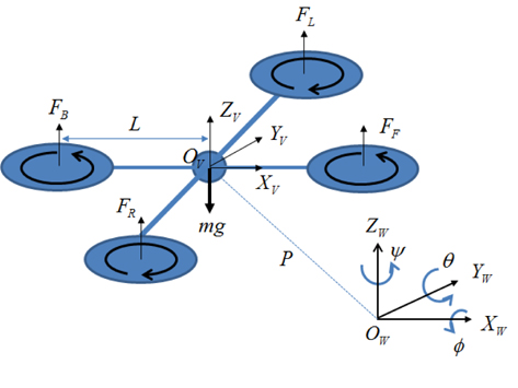
The quad-rotor system has four rotors and propellers, as shown in Figure 1. A pair of propellers rotates in the clockwise direction (
[Table 1.] Motion attained by controlling rotor speed
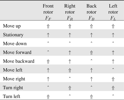
Motion attained by controlling rotor speed
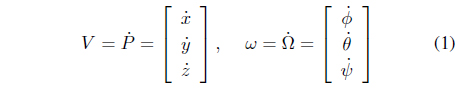
The coordinates of the quad-rotor system (
Changing the speed of each rotor generates translational movement
where
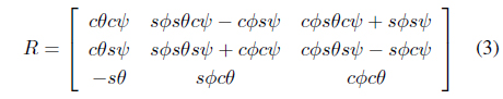
The linear velocity

where

where
Therefore, the linear velocity in the vehicle coordinate is found to be

where
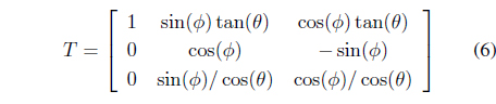
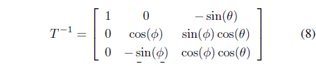
The angular velocity is given by

where

Conversely, the angular velocity of the vehicle frame can be obtained from Eq. (5) as
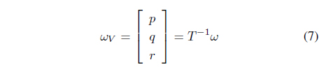
where
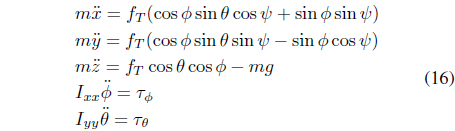
The translational motion equation under the influence of gravity force is defined as

where
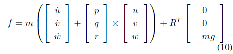
where
Solving Eq. (10) for
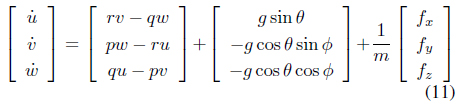
Note that
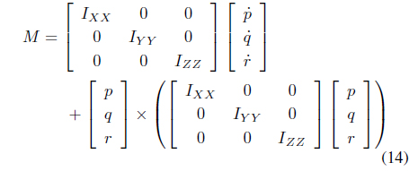
In the same way, the moment equation can be described as

where is the moment force and

where
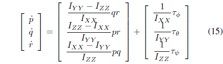
Substituting Eqs. (7) and (13) into Eq. (12) yields

Rearranging Eq. (14) with respect to

It is convenient to represent dynamic Eqs. (11) and (15), specified for the vehicle frame, into a global frame through relationship Eq. (2). The dynamic equation in the global frame, assuming that the Coriolis terms and gyroscopic effects can be neglected, yields
During hovering, the thrust force is assumed to be proportional to the square of propeller’s rotational speed, that is,

where

where
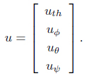
Although we have six variables to represent the system, we have only four inputs, making the quad-rotor an underactuated system. We regard the elevationz, roll, pitch, and yaw angles (

where
The angle of the quad-rotor system is regulated by controlling the velocity of each rotor. The direction of movement of the system is determined by combining the magnitudes of each rotor velocity. Although there are six variables for describing a quad-rotor system, there are only four actuators, which means that control of all six variables is difficult.
The linearized dynamics for the attitude control can be given from Eq. (16) as
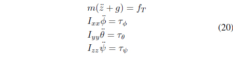
Thus, basic movements such as reaching a certain altitude and hovering while adopting a specific attitude can be considered. The hovering motion is related to the control of the roll and pitch angles, and the attainment of altitude is related to the control of the thrust force. Since a quad-rotor system is a symmetrical structure, yaw angle control is not considered seriously in this case.
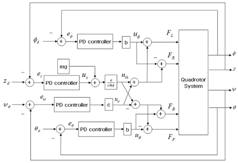
From the roll and pitch control inputs, the force input to each rotor can be determined. Each rotor force is described as

where
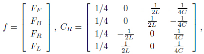
and

In this case,
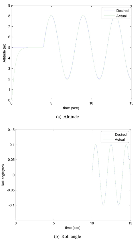
Based on the control block diagram shown in Figure 2, we performed a simulation study. We control the altitude and three angles.
The desired trajectories for the attitude control are given differently with respect to the time range.
i) 0 ~ 4s: zd = 5m, ϕd = 0, θd = 0, 𝜓d = 0 ii) 4 ~ 10s: zd = 5 + 3 sin(2π4t)m, ϕd = 0, θd = 0, 𝜓d = 0 iii) 10 ~ 15s: zd = 5 + 3 sin(2π0.25t)m, ϕd = 0.1 sin(2π0.5t), θd = 0, 𝜓d = 0
Table 2 lists the controller gains. The attitude control performances are shown in Figure 3. We see that the quad-rotor system follows the desired trajectory well.
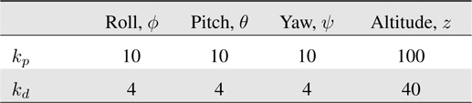
Controller gains
4. Design of Small Quad-Rotor System
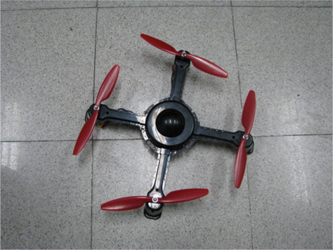
Figure 4 shows the actual small quad-rotor system. The body frame is casted. As the control hardware, AVR is used rather than DSP to reduce the cost.
The sampling time is 4 ms. All of the hardware and sensors are located in the center of the unit. For angle detection, a gyro and an accelerometer are used.
Table 3 lists the specifications of the small quad rotor system. The total mass is 0.95 kg and the maximum thrust is 2 kg.
[Table 3.] Specification of small quad rotor system
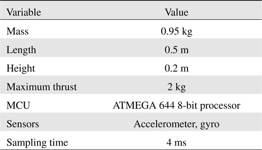
Specification of small quad rotor system
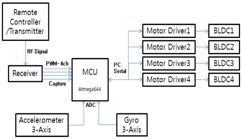
Figure 5 is an overall block diagram of the control hardware. The 8-bit microprocessor performs all of the calculations: control signals, sensor signals, and communication.
5.1 Computing Algorithms for Angles
To obtain the roll and pitch angles, a 3-axis gyro and 3-axis accelerometer are used. The following equations are used to obtain the roll and pitch angles from the accelerometer measurements.

where
Thus, computing Eq. (22) is a burden for an 8-bit processor, since tan−1 and √ operations require the math library and they are calculated based on the floating point data format. This leads to the computational limitation of the processor since the inherent processor cannot handle those computations within an acceptable sampling time. Therefore, the approximation of those mathematical operations is required to approximate the necessary mathematical functions.
5.1.1 Square Root Operation
The square operation can be approximated and obtained by applying Newton’s method through several iterations. Eq. (23) defines the relationship of the square operation. Given value a, value b can be calculated as follows.

Newton’s method is given as

Reformulating Eq. (23) into Eq. (24) yields the update equation.

where
Finally, the value of b can be obtained iteratively.
5.1.2 tan−1 Operation
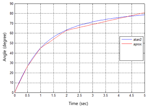
For the tan−1 operation, a table lookup method is used to match the real values of tan−1 with several linear functions within the range of useful angles.
Although there are mismatch errors resulting from the approximation process, these errors are small and can be neglected for real applications. Figure 6 shows the approximation of the
5.1.3 Integer Operation
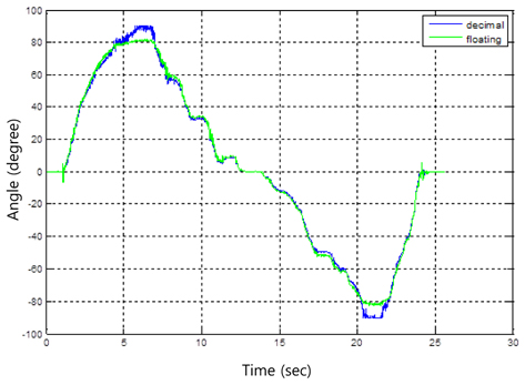
Another consideration is the use of the integer operation rather than the floating point format for numerical calculations. For example, a typical IIR filter calculation can be performed as Eq. (26) for the floating point format that is not permitted by processors with low computational power. Therefore, the integer-based operations in Eq. (27) should be performed by accepting lower computing accuracy.


Within the useful range of angles, namely, from 0° to ±90°, the approximated integer operation is compared with the floating point operation shown in Figure 7. The two operations are similar except around ±90° where there is a slight mismatch between the two operations.
5.2 Complementary Filtering Method
We measured the roll and pitch angles using an accelerometer and a gyro sensor. Since the accuracy of the sensors is poor due to the noisy environment, we applied two-stage filtering. The first-stage filtering involves the use of a complementary filter to maximize the filter characteristics. Then, the second stage filtering technique uses a Kalman filter after the complementary filter to suppress the effects of noise, as shown in Figure 8.
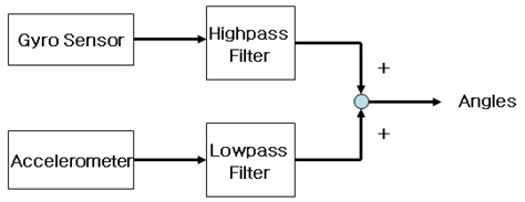
We designed filters that combined the two low-cost sensors: a gyro sensor and an accelerometer. We combine the two sensors as a complementary filter to obtain more accurate angle measurements. The complementary filter consists of a low-pass filter for the accelerometer and a high-pass filter for the gyro sensor. The filtered outputs are added together to estimate the value, as shown in Figure 9.
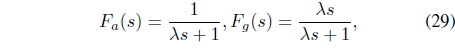
When the sensor transfer functions are given for the accelerometer as

where
Then, each filter of

where
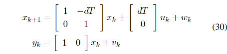
The Kalman filter equation for the angle measurement is given by [21, 22]

where

and
The conventional Kalman filter requires several repetitive steps to estimate states Eq. (31) to Eq. (35).
Time update:


Measurement update:


where
However, the computation of the Kalman filter is a considerable burden for an 8-bit microprocessor. Although the Kalman filtering method normally requires an iterative procedure to update the state correctly, a simplified version can be used. Instead of using all the steps of the Kalman filtering algorithm, a simplified process can be employed whereby the Kalman gain is fixed. In this case, the updates of Eqs. (32, 33, 35) are not required. Therefore, the form of the simplified Kalman filter algorithm will be as follows:
Time update :

Measurement update :

where the Kalman gain
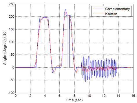
We conducted a filtering test based on the aforementioned simplified algorithms. The result of one typical filtering test is shown in Figure 10. The results of the single-stage and two-stage filter design technique are compared. The filtered signal, after being passed through the complementary filter, is compared with the signals output from the Kalman filter after the complementary filter. We can clearly see that the signals output from the two-stage filtering method, after being passed through the complementary and Kalman filters, are more stable.
5.5 Overall Hardware Structure
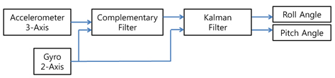
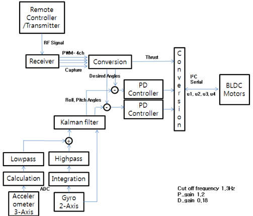
The signals obtained from the filtering algorithms were used in the control algorithms. Figure 11 shows the connection between the control and the filtering block diagram. The roll and pitch angles are measured by a gyro and an accelerometer, and those signals are fused with the complementary filter, for which the cutoff frequency is set to 1.3 Hz. Then, the signals are passed through the Kalman filter.
The filtered signals are used for PD controllers and the PD gains are set to 1.2 and 0.18 for the proportional and derivative gain, respectively. Then, the control torque applied to each rotor is calculated by Eq. (19).
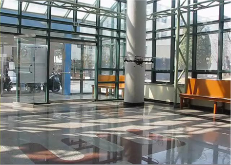
After implementing the hardware and software under the aforementioned constraints, flying tests were conducted for real operations. Firstly, a flying test for the small quad-rotor system was performed inside a building to minimize disturbances such as that presented by wind.
Figure 12 shows a flying demonstration controlled by a joystick through a remote controller.
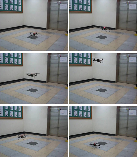
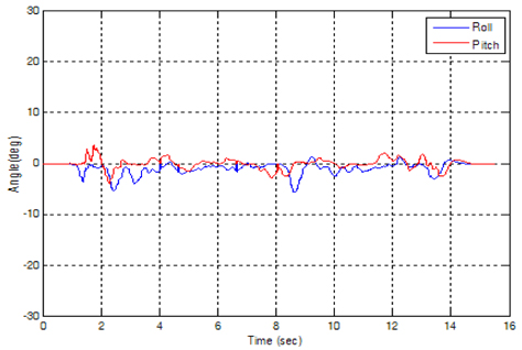
Another indoor flying test was conducted in a small space. Figure 13 illustrates an actual indoor flying task where the quad-rotor elevates from the floor and then lands on the floor. All of the trajectory commands are issued by the remote controller. The corresponding roll and pitch angle plots are shown in Figure 14. We can clearly see that the roll and pitch angles are well balanced. The oscillation errors are within about ±5°.
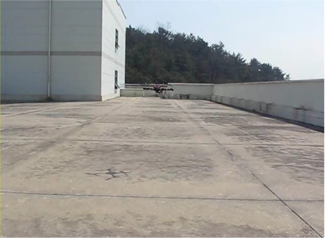
After adjusting the control parameters for stable flying in the indoor environment, the quad-rotor system was tested in an outdoor environment (on the roof of a building). Figure 15 illustrates the actual flying movement. The quad-rotor system was controlled by an operator.
We have presented the implementation of a small quad-rotor system under several practical constraints of minimizing the total cost. Changing the main control hardware from a DSP to an AVR limits the computational ability of the filtering and control algorithms. To satisfy the desired sampling time, the required mathematical functions are simplified and approximated. In addition, a simplified version of the Kalman filtering algorithm is presented and used for actual system control. Actual flying demonstrations in both indoor and outdoor environments confirmed the functionality of the small quad-rotor system using approximated calculations for the algorithms.
No potential conflict of interest relevant to this article was reported.