Laser-induced breakdown spectroscopy (LIBS) is an atomic emission spectroscopy that uses a highly energetic fast laser pulse focused on the sample to form plasma, the ablated material breaks down into atomic species and excited ionic species. LIBS can analyze any matter regardless of its physical state, be it gas, liquid or solid. LIBS has gained great interest for qualitative and quantitative analysis for many materials including, nano-ceramics, polymers semiconductors etc, because of its ease of use, fast response and high sensitivity [1-4], Furthermore, remote analysis of the full elemental composition of a sample is achieved via properly optimized LIBS technique [3]. By means of in-situ analysis, both the complexity and the cross contamination of the detection process could be minimized [5]. LIBS is a quite straightforward plasma spectroscopy technology, using high intensity laser pulses (~1 TW/cm²) focused on a sample, thus producing plasma and ablating a very small amount of material. The produced plasma expands then cools with time, and the characteristic atomic emission lines of the elemental content in the sample could be observed. The spectral lines’ intensities for particular elements are proportional to the elements’ concentration in the sample. In recent years, the growing technique of LIBS has been applied broadly with increasing success in the qualitative and quantitative analyses of soil components and additives with relevant simplification of the conventional methodologies [1-4]. However, the LIBS technique still needs additional verification before it can be implemented effectively in environmental soil analyses.

Soils represent a crucial constituent in the biogeochemical carbon cycle, and their abilities to store carbon are higher than those of biomass plants by several times. Hence, quantification of soil carbon in field conditions has a significant challenge corresponding to global climatic changes and the carbon cycle. Recently, Da Silva et al. [6] succeeded in calibrating a portable LIBS system to execute quantitative measurements of carbon content in a tropical soil sample. Even though their LIBS system was used for qualitative elemental analyses with no prior sample treatment, the results were obtained directly. The obtained results demonstrate the significant impact of implementing portable LIBS systems for both qualitative and quantitative analysis of carbon content in tropical soils. Santos Jr. et al. [7] aimed to validate the capability of LIBS to detect cadmium ions in soils since cadmium is considered as a high toxicity potential agent and can be accumulated in the living organisms. They established a computerized fast pre-processing series of algorithms for converting a sequence of several hundreds of LIBS spectra collected from a single target into an accurate enhanced spectrum. The observed spectrum provides a procedure to determine its spectral elements and a series of calibration-curves using multi-cation sulfates and standard hydrous. They were capable to observe the concentrations of Ca, S, Al, K, Mg, Fe, Na, H, and O in sulfates, along with the degrees of hydration of Mg-sulfates and Ca-sulfates, from LIBS spectra [7].

In the present study, we aim to use the LIBS technique to investigate soil samples that are collected from deserts in various locations around Riyadh city in Saudi Arabia. The spectra of major and trace elemental compositions of collected soil samples are studied. The time dependence of electron temperature and density for the observed plasma on the soil matrix is also investigated.

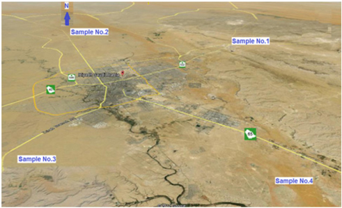
In the present work, four different soil samples were collected from four various locations from desert around Riyadh city. Sample-1 (ES) was collected from the east, 25 Km from the center of Riyadh. Sample-2 (NS) was collected from the north, 20 Km from the center of Riyadh. Sample-3 (WS) was collected from the east, 30 Km from the center of Riyadh. Sample-4 (SS) was collected from the south 50 Km from the center of Riyadh and close to Al-Kharj city. Locations of the samples are shown in the map given in Fig. 1. These samples were ground then pressed into pellets of 30 mm diameters using pressure of 20 tons for 15 minutes.

The schematic diagram of the LIBS experimental setup was shown elsewhere before in detail [5]. Briefly, in the current setup the LIBS experiment was carried out using a compact LIBS system spectrolaser model 7000 from Laser Analysis Technologies, Australia. The latter is a complete integrated system containing a Nd:YAG laser as an excitation source, high resolution optical spectrograph, focusing optics, sample chamber, optical fibers, and CCD detectors with special data acquisition software. The excitation laser source is a high power Q-switched pulsed Nd:YAG of 7 ns pulse at the first harmonic 1,064 nm for energy ranges 5-300 mJ and repetition rate of 10 Hz. The system could focus on a fresh region of the sample through an x-y translation stage for the successive laser pulses. In the current study, laser energy of 50 mJ has been used with a CDD detector of a varied delay time and fixed gate width of 1 μs (the gate width could not be changed for that system). Using a convex lens of 45 mm focal length, the laser beam was focused at the target to ablate material from the sample surface and produce a plasma plume. A bundle of optical fiber (600 μm in diameter) was used to collect the radiation emitted by the generated plasma. This collected light was then analyzed using a high-resolution spectrometer (~0.1 nm FWHM) attached to a gated CCD. To minimize the noise, an average of 10 collected spectra was recorded for each LIBS spectrum, for the full active range from 190~1,100 nm.

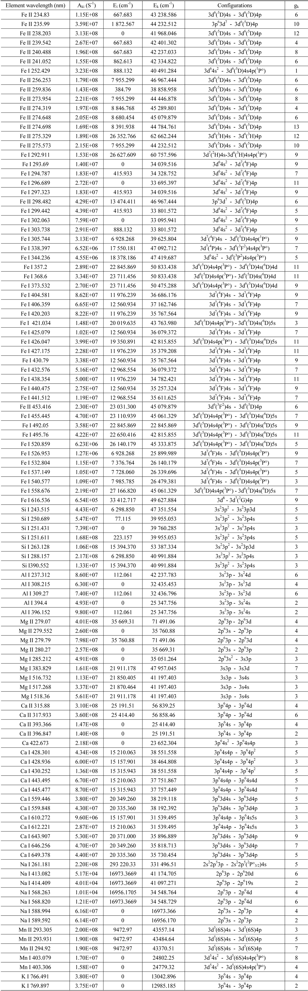
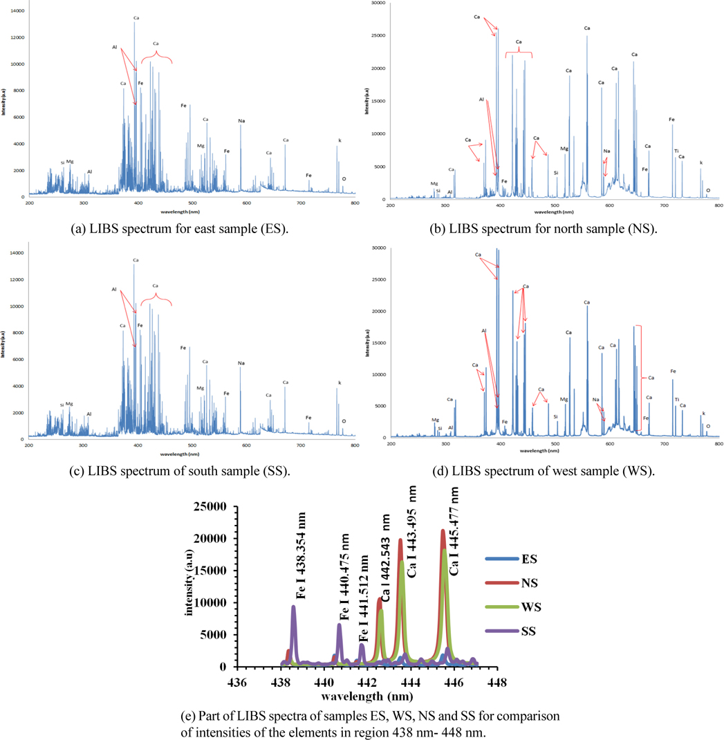
Typical LIBS soil spectra for the spectral range from 200 nm to 800 nm are shown in Figs. 2(a)-(d), for ES, NS, SS, and WS soil samples respectively, using spectrolaser software provided with the “Spectrolaser” LIBS system. The obtained results revealed that the concentration of elemental content of the soil samples varied from one desert area to another. This is clear by comparing the relative intensities of the spectral lines for the four samples as shown in Fig. 2(e). The latter figure demonstrates the observed spectral lines’ intensities for iron and calcium in the spectral region 438 nm - 448 nm include: Fe I 438.354 nm, Fe I 440.475 nm, Fe I 441.512 nm and Ca I 442.543 nm, Ca I 443.495 nm, Ca I 445.477 nm. Using a fixed laser energy value, the relative intensities for iron lines are higher for SS samples than for others while the relative intensities for calcium lines are high for NS, WS samples compared to other samples. Since the change of the line intensity is associated with change of the elemental concentration; the observed result revealed that the concentration of elemental content of soil varied from one area to another. A list of 106 resolved spectral lines of the elements along with all spectroscopic data for the investigated samples is given in Table 1.

The ablated mass of the sample depends on the physical properties of the sample, the absorption of the incident laser beam radiation by the surface, the plasma-shielding, which is associated with the electron density of the plasma, and the laser flounce [14-15]. Hence, studying the plasma temperature and the density of plasma species is essential for the understanding of the dynamics of ionization, the dissociation-atomization, and excitation processes occurring in the plasma [9]. The population density of atomic electronic and ionic states could be expressed using the Boltzmann distribution function if the laser induced-plasma fulfills the local thermodynamic equilibrium (LTE) condition. For low-density optically thin plasma, the effects due to re-absorption of plasma emission can be neglected [2]. Consequently, the intensity of the emitted spectral line (I) can be determined from the fractional population of the corresponding energy level of a particular element in the plasma. The plasma electron temperature can be calculated via the excitation state intensity of the emitted spectral line (I) using the well-known Boltzmann equation [17], if the plasma satisfies the LTE condition as:

where λ is the wavelength (cm), g_k is the statisticalweight for the upper level, A_ki is the transition probability (s^-1), T is the plasma electron temperature (Kelvin), E_k is the excited level energy (cm^-1), U (T) is the partition function, K is the Boltzmann constant, C is the species concentration and F is an experimental factor.

From the slope of the plot of the left hand side of Eq. (1) vs. the excited level energy E_k, the plasma temperature T can be calculated. Throughout the initial steps of plasma formation, an intense continuum (Bremsstrahlung radiation) predominates in the emitted spectrum. Thus, many heavily-broadened ionic lines of the elements present are overlaid. The main physical causes of the spectral line-broadening are the Stark broadening and the Doppler broadening. Stark broadening due to collisions of charged species is taking place at this early period. Additionally, the spectral lines of the excited neutral atoms are rather weak, and they regularly coincide with the strong ionic lines. Therefore, the isolation and observation of neutral lines are difficult [5].

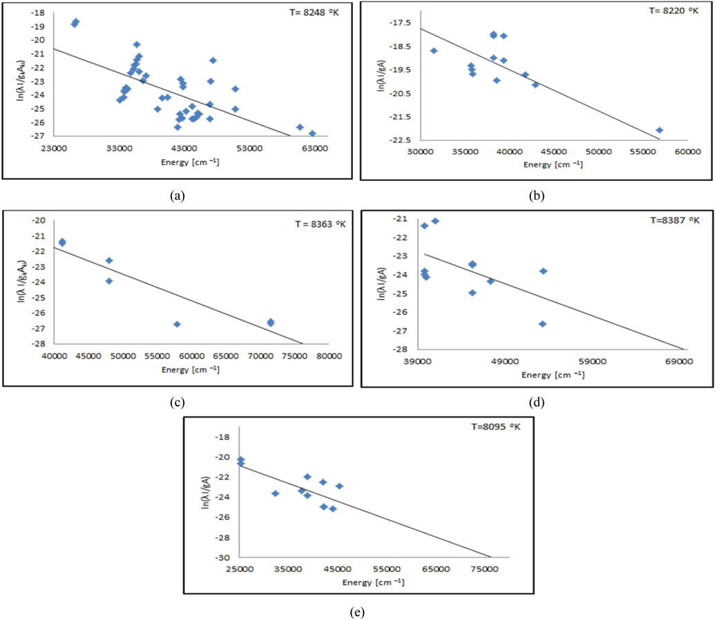
Thus, the continuum can be avoided by longer delay detection time. Nevertheless, each particular spectral-line reveals different temporal evolution that relates to specific atomic energy level of the corresponding element. In order to calculate Te plasma electron temperature of the soil samples, the Boltzmann plot was determined for the resolved spectral lines of the elemental contents (Ca, Fe, Al, Si and Mg). Then an average value of all temperature values of corresponding elements in each sample was determined and listed in Table 2. The Boltzmann graph was plotted between ln (Iλ/gA) and (E in cm^-1) according to the formula given in equation (1). The Boltzmann graphs for Fe, Ca, Al, Si and Mg elements in NS and NE samples are depicted in Figs. 3(a)-(d).

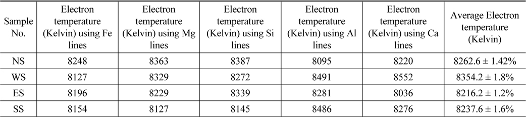
The plasma electron-density N_e is observed by measuring the fundamental width at half maximum FWHM (Δλ_1/2) broadening of an appropriate emission line of the laser-plasma spectrum. The spectral width of Stark broadening for an elemental-emission line depends on the electronic density[2]. For a non-H-like spectral line, the Ne (in cm^-3) is determined from the (Δλ_1/2) of the line from the following formula [9-13] ;

where w (nm) is the Stark broadening value or electron impact parameter [10]. This formula is commonly used for considering N_e of a plasma produced from solid targets [11]. Measurements of FWHM (Δλ_1/2) for Mg (285.212 nm), Ca (422.673 nm), Si (390.552 nm), Al (308.215 nm), and Na (589.592 nm) are shown in Figs. 4(a)-(f), respectively.

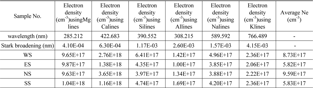
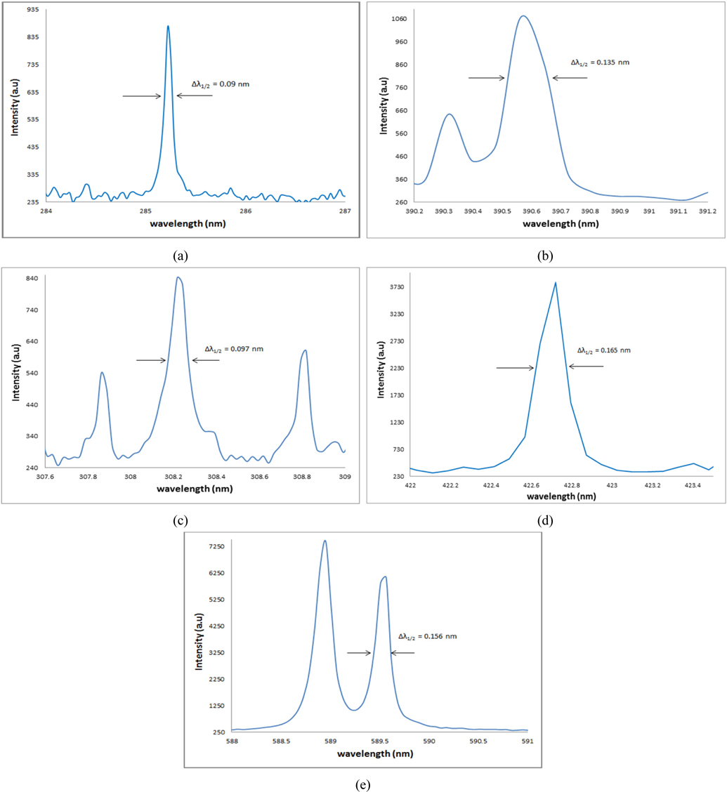
The Stark broadening values used to calculate the electronic density of detected elements in this work are given in Table 3 from Ref [10]. Electron density Ne calculated for Mg (285.212 nm), Ca (422.673nm), Si (390.552 nm), Al (308.215 nm), and Na (589.592 nm) for all samples are given in Table 3 as well. The higher Ne values for calcium and magnesium are expected to be due to additional intensity values for resonance lines that experience self-absorption, which returns broader lines. Fig. 2. above demonstrated that the sodium concentration is very high compare to other elements that Ca and Mg. These elements are expected to be major elements represent 30-40% of the content of our collected samples. The rest of Ne values for the other elements have the same order of magnitude with error of 10-20%.

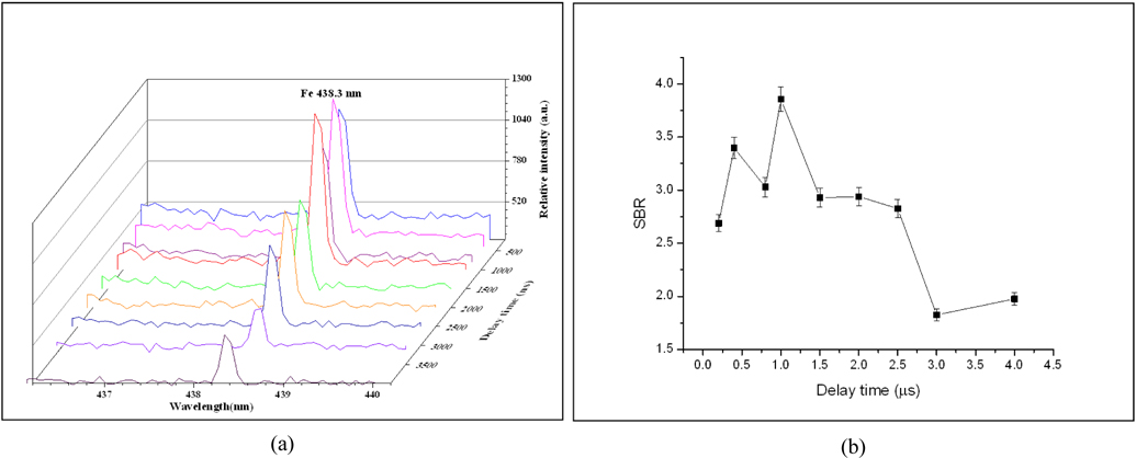
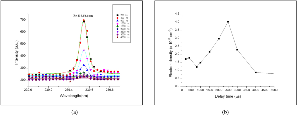
The time resolved LIBS measurements have been applied for the soil samples using the same experimental conditions (mentioned above) under a varying delay time. Figs. 5(a), (b) demonstrates the variation of Fe 438.354 nm atomic line intensity and its signal-to-baseline ratio (SBR) with delay times from 200 ns up to 4 μs for soil sample NS. The figure revealed that the maximum SBR for the 438.3 nm line reached a maximum value at 1 μs delay time. For studying the time resolved plasma characteristics of our soil sample, we have to select suitable resolved lines with the needed spectroscopic data for any of the sample elemental content as represented before in Table 2. For iron, we used the resolved ionic line Fe 239.542 nm with its Stark broadening value (1.17 × 10^-02 nm) from ref. [16] to determine the plasma electron density Ne using Eq. (2).

Figure 6(a), represents the LLorentzian curve fitting of Fe 239.542 nm line to determine the variation of FWHM with delay time. The temporal behavior of the electron density, shown in Fig. 6(b), demonstrates the effect of collisional processes by the value of the electron density which increases gradually at the early time of the plasma evolution, till it reaches a maximum value, while the recombination processes are recognized at longer delay time. It is found that Ne reaches its maximum value of 4.0 × 10¹⁷ cm^-3 at 2.5 μs then cooling increased with time.

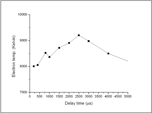
For the plasma electron temperature Te, we used the resolved lines listed at Table 1 to determine the Boltzmann plot as represented before in Fig. 3(a) using Boltzmann Eq. (1). Fig. 7. demonstrates the variation of the plasma electron temperature of the Fe with delay time. The later figure revealed that Te has a temporal profile similar to Ne, i.e. Te increases with the delay time and reaches its maximum value of 9,235 K at 2.5 μs then cooling increased with time. This performance of plasma is different from metallic materials which have much faster recombination processes at early times followed by slow dynamics at longer ones as founded by our group before [11].

Finally, by considering the plasma temperature and the electron density we can examine the validity of the local thermodynamic equilibrium (LTE) assumption by considering the criterion given by McWhirter [17].

The lower limit condition for electron density at which the plasma can be considered in LTE is:

T is the plasma temperature, and ΔE is the largest transitional energy for which the condition lasts [18].

In the present study ΔE = 5.278 eV for Fe (as listed in Table 1) and the electron density lower limit value given by Eq. (3) is 1.86 × 10¹⁶ cm^-3. The experimentally calculated electron density values (Table 3) are greater than this value, which is agreed with the assumption that the LTE predominates in the plasma.

This paper encompasses the application of LIBS to soil analysis in the desert and the composed plasma characterization. More than hundreds of spectral lines are highly resolved for elemental composition of natural soil samples. The observed results indicated that electron temperature and density of the observed plasma depend on the sample matrix. These, consequently, alter the spectral characteristics of each element in the same soil matrix. The time resolved measurements of plasma parameters revealed that both Te, and Ne reach maximum values at 2.5 μs then slow recombination processes take place at later times. This plasma performance is contrasted with the fast plasma recombination of metallic materials found before. Furthermore, the LTE conditions are verified for the observed plasma measurements. This study is important for improving LIBS as a calibration-free technique in environmental applications. The later could be achieved in the future by measuring plasma parameters of only a single element as an indicator to recognize the desert soil matrix composition without analyzing that matrix and without ordinary calibration curves, thus saving a lot of time and effort.