White-light phase-shifting interferometry (WLPSI) proposed by [2] and [3, 4] has high resolution over long distances. WLPSI, however, cannot overcome the limitation of phaseambiguity entirely, because it can also detect the fringe order incorrectly due to the problem of phase ambiguity. In order to address this issue, a specific strategy has been required to determine the correct fringe order in relation to WLPSI.
Previous research related to determining of fringe order was done by [3, 4], [5, 6] and [7]. This work, however, yielded solutions only for limited samples. [8] suggested a method to determine the fringe order by phase unwrapping, though it is not sufficient in practical applications given undesirable conditions such as noise, diffraction and steep angles.
In this paper, a new algorithm that corrects errors in fringe-order determinations is proposed. Prior to the phase unwrapping process, parameters such as the decouple factor and the connectivity are introduced and calculated. The decouple factor can compensate for the effect of a phase delay. As the connectivity contains information on the edges at which phase unwrapping is prohibited, it is possible to suppress excessive phase unwrapping.
To verify the performance of the algorithm, a simulation was performed with the virtual step height under noise. Some specimens such as step height standard and a column spacer with a steep angle are also measured with a Mirau interference microscope, after which the algorithm is shown to be effective and robust.
2.1. Introduction of the Decouple Factor
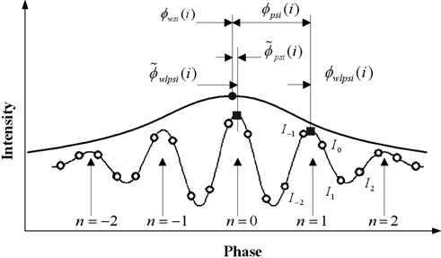
The WLPSI equation using both the phase of white-light scanning interferometry (WSI) and the phase of phase shifting interferometry (PSI) is
where 𝝓
When we assume the fringe order
where is the phase from WLPSI when the fringe order
From Eq. (3), a reasonable proposition can be made such that the fringe order can be assigned as the same fringe order of , when the both sides of Eq. (3) are phase-unwrapped. We can express this condition as follows;
For neighboring points,
where
Equation (4), however, cannot be met at all points due to practical measurement conditions such as noise, diffraction and s steep angle. Therefore, 𝝓
where 𝝓
If we can calculate 𝝓
2.2. Calculation of the Decouple Factor
In this section, we propose a method to calculate the decouple factor in practical applications. From our practical application, 𝝓
Then Eq. (4) can be rewritten considering Eq. (5) and Eq. (6).
After Eq. (5) is applied to Eq. (7),
Let △𝝓
Apply Eq. (9) into Eq. (8),
From Eq. (10),△𝝓
For a valid △𝝓
In order to calculate the decouple factor 𝝓
will be used instead of △𝝓
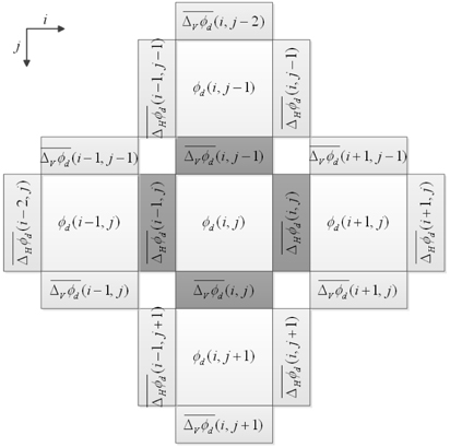
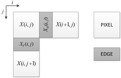
For an easy explanation, we consider the pixel and edge figure shown in Fig. 2. The pixel figure indicates the value defined at the pixel, in this case , , and 𝝓
We extend the previous equations from a one dimensional case to a two dimensional case as shown in Fig. 3. In a two dimensional case, one point has four edges on the upper, lower, left, and right sides. The difference values,
We already know the values of 𝝓
Next, we explain how to calculate the decouple factor 𝝓
Each equation has one 𝝓
After this strategy is applied once more to the second term in Eq. (21), Eq. (21) is rewritten as follows;
The third term in Eq. (22) has a constant This effect is almost 1% of the total effect. This term can be ignored.
2.3. Introduction of the Concept of Connectivity
We introduce the concept of connectivity in order to consider the disconnected edges, serving two purposes. First, the connectivity can change the decouple factor 𝝓
The connectivity can be given at all edges as follows;
The connectivity initially is assigned as one at all edges, and then changed to a zero under the next three conditions
1. At the boundary of the measurement area: that is, i=0, i= Mx; j=0, j=My. At the edges of an point where the light intensity signal cannot be obtained.3. If the difference in between the neighboring points exceed over 5π , as mentioned in relation to Eq. (7).
where
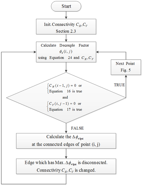
2.4. Iterative Correction of the Decouple Factor and the Connectivity
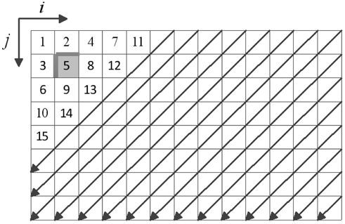
We check and correct the decouple factor and the connectivity using the steps in Fig. 4and Fig. 5, where Fig. 4 shows a flow chart for checking the decouple factor and changing the connectivity at each pixel and Fig. 5 shows when using this flow chart. First 𝝓
The remaining final step involves simply unwrapping the phase. In this paper, we use [10]a phase unwrapping method, which is modified to consider the decouple factor and the connectivity. A modified version of Herráez’s method uses a phase of , which is corrected with the decouple factor in place of the original phase 𝝓
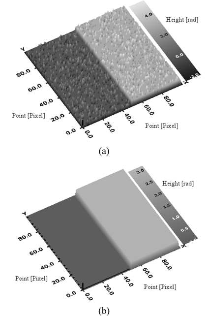
To examine the robustness to noise of our algorithm, a simulation was performed using the following procedure. The virtual step height with white noise in a range of -
where
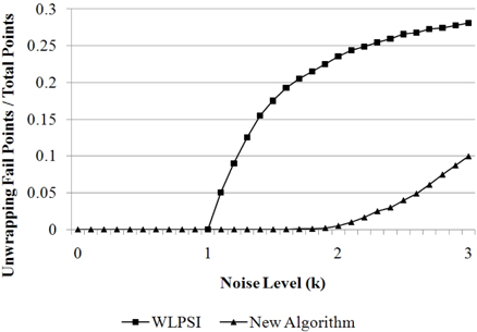
When the noise level
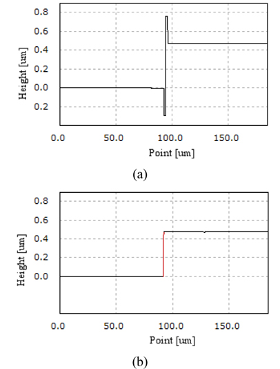
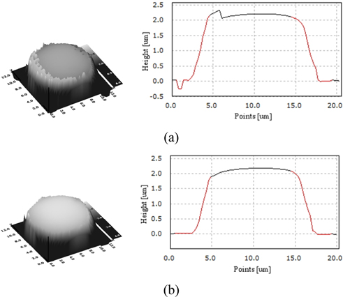
When the measurement height is identical to or lower than the wavelength of the light source, the measurement result can be distorted by diffraction at the sharp edge of the step height, as noted in earlier research by, for instance, [5]. We measured the step height standard, VLSI SHS-4500, at a height of 470.3 nm, which is quite close to the wavelength of light, with a 50X Mirau interference microscope. We intend to compare the result after we intentionally create the worst case with a large phase delay. In that case, the apparatus has a high-magnification lens and uses a Mirau-type lens. As shown in Fig. 8(a), we observed that the measured result was distorted at the edge of the step height standard without our fringe-order determination method. However as shown in Fig. 8(b), the measurement result was not distorted.
As shown in Fig. 9, another measurement test was performed with a Mirau interference microscope. We measured the LCD column spacer sample as shown in Fig. 9, which has a gradient on its surface with a phase delay of
In this paper, a new algorithm is proposed for the fringe-order determination in the white light phase-shifting interferometry to compensate for the phase delay and to suppress excessive phase unwrapping to overcome the phase ambiguity problem.
(1)A decouple factor is proposed to compensate for the phase delay. When the phase is compensated for by the decouple factor prior to unwrapping, the WLPSI result can be successfully unwrapped, using the proposed Eq. (24) for calculating the decouple factor at all points. (2)The concept of connectivity is proposed to suppress excessive phase unwrapping. The connectivity is defined in the vertical and the horizontal directions, and proper initial connectivity values are devised beforehand as explained in Section 2.3. This process allows the determination of the edges at which phase unwrapping is prohibited.(3)The decouple factor and the connectivity are successfully calculated and corrected according to the proposed flow chart shown in Fig. 4.(4)We performed a simulation under noise to verify the proposed method. The result showed that our method can reduce the errors induced by diffraction at a low step height close to the wavelength of light. We also measured a sample with a steep angle, with the result demonstrating that our method can successfully perform phase unwrapping for a phase delay of more than π.(5)The proposed algorithm is found to be very robust against noise, diffraction, and the angle of the surface through measurement tests using white-light phaseshifting interferometry.
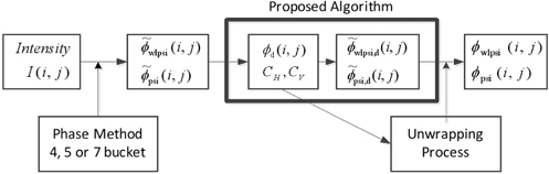
The proposed algorithm is summarized as shown in Fig. 10. This algorithm adds the decouple factor and the connectivity to the conventional WLPSI process which has the phaseunwrapping process. So our algorithm can be used in the conventional WLPSI which uses any phase method like the 4 bucket, 5 bucket and 7 bucket algorithm. The calculating time according to this algorithm is small. Some initial value calculation time and the flow chart calculation time of Fig. 4 are needed additionally. The flow chart calculation of Fig. 4 was processed one time for each pixel. So the number of total calculations is the same as the total number of pixels.