One of the most essential technologies for operating unmanned vehicles is to compute navigation information, including the position, velocity, and attitude of a vehicle. A number of autonomous vehicles have been developed, such as a guided weapon system, UGV (Unmanned Ground Vehicle), USV (Unmanned Surface Vehicle), and UAV (Unmanned Aerial Vehicle), for surveillance, reconnaissance, and many other dangerous and difficult missions. For autonomously operating these unmanned vehicles, many navigation sensors and systems are used, for example IMU (Inertial Measurement Unit), GNSS (Global Navigation Satellite System), vision sensor, LiDAR (Light Detection and Ranging), magnetometer, barometer, etc. Among these, GNSS is an essential system, which can provide accurate absolute position information of a vehicle within certain error bounds, as well as velocity and time information. In particular, the GPS/INS integrated system, which can provide a drift-free and accurate solution of a highly dynamic vehicle, by using GPS (Global Positioning System) satellite signals to correct the solution from an Inertial Navigation System (INS), has been widely used on ground and aerial vehicles, for precise navigation purposes.
However, the performance of the GNSS-based navigation system is likely to be affected by satellite observation environments, since the system cannot provide the navigation solution in poor environments. For example, when a vehicle is downtown or in cloud forests, the number of visible satellites decreases drastically, and multipath error is very likely to occur. Furthermore, under indoor or jamming environments, the satellite navigation system cannot be used. To overcome the unavailability problem of GNSS, various researches have been studied. Among those, research on the integration of IMU and vision sensor is notable [1-3]. The research is generally based on SLAM (Simultaneous Localization and Mapping) technologies. The most representative way is to use feature points, which are easily distinguishable from other pixel points of the captured image [4-9]. The navigation solution of the feature point-based SLAM system has generally a diverging property, since the navigation algorithm inherently relies on the accuracy of both the feature point position estimates, and vehicle estimates, which tend to deteriorate, due to mutual error accumulations. Also, it is difficult to detect and track high-quality feature points in unstructured environments where no previously known landmark exists.
Meanwhile, an optical flow that represents the motion of pixels was also utilized in vision-aided navigation systems [10, 11, 13-14]. In [11], optical flow vectors were used for road navigation, to estimate the forward velocity and heading angle of a car, and detect moving cars on the road. Additionally, it was applied to the autonomous flight control of a MAV (Micro Air Vehicle) in indoor corridor environments, and autonomous take-off and landing of a small-scale UAV [13, 14]. However, it is rarely reported that optical flow is directly adopted for estimating 6 DoF (Degree of Freedom) navigation solutions.
In a different approach from vision-based navigation systems, the LiDAR-based navigation system has been independently developed to deal with GNSS-denied environments. As a result, a localization and mapping system for mobile robots and multi-rotors has been developed. In [15], scan matching based two-dimensional SLAM and INS are loosely integrated, based on an EKF (extended Kalman filter) framework, and the developed system is applied to UAV, USV and small handheld embedded systems. However, the designed system considers two-dimensional motion only in the limited environment where specific obstacles are within the range of LiDAR. Thus, it cannot be applied in unstructured outdoor environments, such as open terrain.
In a few works, research on SLAM combining both vision and LiDAR sensor were investigated. For instance, IR scanner, vision sensors and encoders were simultaneously integrated, based on a particle filter framework for mobile robot localization, with the assumption of previously known map information. Besides, research on detecting moving cars and pedestrians, and research on indoor path planning of UAV were developed, by combining computer vision processing results with LiDAR measurements [16-18]. Nevertheless, these efforts put most emphasis on detecting and localizing possible obstacles via heterogeneous sensor fusion, and thus suffered from generating extensive status information of the host vehicles. Consequently, a literature survey reveals that no published result presents direct integration of vision sensor and LiDAR within an INS mechanization scheme, for a complete navigation solution for unstructured outdoor environments.
In this paper, we present a Vision/LiDAR aided integrated navigation system, for an environment where 1) GNSS signals cannot be used; 2) the altitude of the ground surface is varying; and 3) there is no known map information. The presented system consists of a mid grade strapdown IMU and a vision/LiDAR system, on a gimbaled platform, onboard the vehicle. The system turns out to provide a reliable navigation solution, by suppressing divergence of the INS error, with the help of vision sensor and LiDAR measurements. In detail, the horizontal velocity error is obtained by correcting the velocity estimate of INS, with that derived from optical flow measurements. In particular, a new piecewise continuous slope model is introduced for the ground, in calculating altitude increment of the proposed measurement model. Basically, range error is obtained by combining the INS solution and attitude compensated range information from LiDAR. In parallel, the height of the ground surface is estimated, which relates to the geometric relation between two boundary LiDAR measurements. Then, the combined error, including range error and ground altitude variation, serves as the true measurement of the vehicle’s altitude change. Finally, the overall integrated navigation system is implemented, based on EKF framework, supported by a simulation study to verify the feasibility of the proposed system.
The rest of the paper is organized as follows: Section 2 describes the concept of the proposed integrated navigation and its coordinate system. In Section 3, the INS error model and sensor model are presented, for constructing the integrated navigation filter. After that, Section 4 provides simulation results, to verify its feasibility in GNSS-denied environments. Finally, Section 5 concludes the paper, with a discussion of our current research.
The proposed integrated navigation system considers its operation onboard a UAV, flying over flat or sloped ground, under GNSS-denied environments. To illustrate the working principle and basic architecture of the proposed system, the sensor integration concept and the adapted coordinate system for the low or mid grade IMU (inertial measurement unit), vision sensor, and LiDAR are presented in this section.
2.1 Concept of the Proposed System
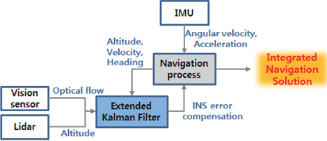
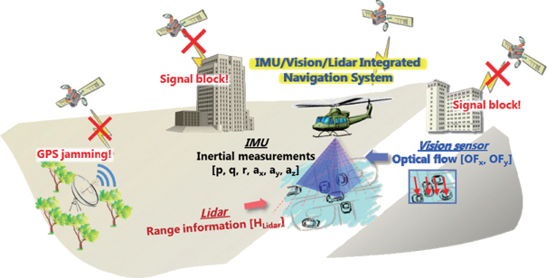
The concept of the proposed integrated navigation system is described in Fig. 1. The system provides a relative navigation solution, with the aid of the vision sensor and LiDAR measurements, when the GNSS signal cannot be used. The IMU operating at a high rate is mounted on the vehicle body, which results in a strapdown INS mechanization. The vision sensor and LiDAR operating at a lower rate than the IMU are mounted on a stabilized twodimensional gimbal system; thus these sensors can keep their sensing axis perpendicular to the local navigation frame, regardless of the vehicle’s roll/pitch motion. Although the GNSS/INS integrated system guarantees a tolerable navigation accuracy in normal conditions, the performance abruptly degrades, as GNSS signal outage occurs. In this background, it is attempted to suppress the rapid divergence of the navigation solution, by compensating INS errors, through the measurements from the vision sensor and LiDAR.
Optical flow vectors representing the motion of pixels are calculated, using consecutive image frames. If it is assumed that the rotational motion of the vehicle is sufficiently negligible, compared with the longitudinal or lateral motion, the optical flow effectively represents the translational motion of the vehicle, because the motion of the vision sensor is not affected by the roll/pitch motion. Therefore, by associating the flow vector with the camera model for coordinate transformation, the horizontal translational velocity can be computed. At the same time, the altitude variation of the ground surface can be calculated, using two range measurements (forward and backward range signal) from the LiDAR, which can be further used to obtain the vehicle’s accurate altitude change on a general sloped ground.
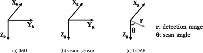
The sensor coordinate system of the three sensors for constructing the presented navigation system is shown in Fig. 2.
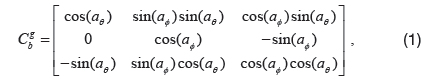
The coordinate system of the IMU is equal to the body frame of the vehicles. The vision sensor and LiDAR are mounted on the two-dimensional gimbal system, which is referenced to the gimbal coordinate system, and aligned with the local navigation frame (NED frame), except for the down axis. In the figure below, the subscript b denotes the body-fixed coordinate system, and the subscript g denotes the gimbal coordinate system. Images from the vision sensor are on the Xg-Yg plane, and the LiDAR provides detection ranges and scan angles on the Xg-Zg scan plane, whose zero degrees scan angle is equal to the Zg axis. Then, the relationship between body-fixed coordinate and gimbal coordinate system can be simply expressed, using the wellknown direction cosine matrix, containing only roll (

3. Integrated Navigation System
The Psi angle approach is used as the INS error model. The error model is the most widely adopted approach, and has been implemented in many tightly coupled integrated systems [19]. The INS error model is shown below.
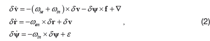
where,
δ r, δ v , δ ψ : Position, velocity, attitude error vectors w.r.t. the navigation frame ωie : Earth rate vector ωin : Angular rate vector of the true coordinate system w.r.t. the inertial frame ωen : Angular rate vector of the true coordinate system w.r.t. the Earth frame ▽ : Accelerometer bias error vector ε : Gyro bias error vector f : Specific force vector
The vision sensor and LiDAR maintain the horizontality condition all the time. Optical flow vectors are modeled using the translation velocity of the vehicle and range information, and the altitude variation is modeled using LiDAR forward/backward range measurements, and their geometrical relations with the ground surface.
3.2.1 Optical Flow Measurement Model
The direction of the optical flow vector is opposite to the direction of the vehicle motion, and its magnitude is proportional to the velocity, and inversely proportional to the relative height between the sensor and ground surface. The simple planar model for the translational velocity matches well with most fixed-wing aircraft flight cases, where no high maneuvering dynamics are assumed [12]. Then, equations (3) and (4) represent an optical flow model, based on a pinhole camera model. In this equation, optical flow is the amount of pixel movement in pixel units.
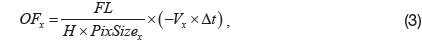
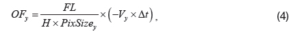
where,
OFx, OFy : Optical flow measurements [pixel] Vx, Vy : Translational velocity w.r.t. the body frame [m/s] △t : Interval time [s] H : Ground height [m] FL : Camera focal length [m] PixSizex, PixSizey : Magnitude of the 1 pixel [m]
Then, the translational velocity in the NED frame is represented by the following equation:
where,
3.2.2 Altitude Measurement Model
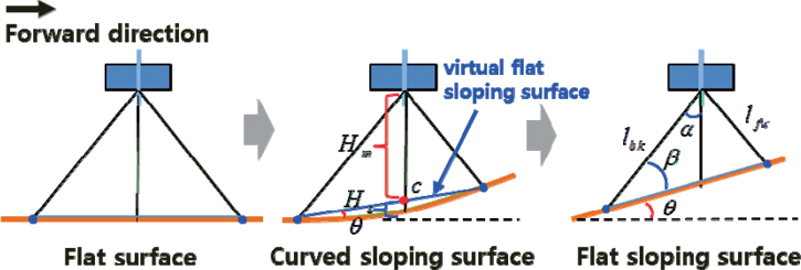
LiDAR can measure the distance to targets, with respect to scanning angles. The detected range at a scan angle of zero degrees represents the vertical distance to the ground surface, since the LiDAR always looks downward, as well as the vision sensor. If the height of the ground surface is not varying, the vertical distance can be simply used as an altitude measurement. But if it is varying, the height of the ground surface should be computed, through a geometric condition. Fig. 3 describes the geometrical relations between the LiDAR measurements and the ground surface.
When it is assumed that the shape of the ground surface is smooth, the type of ground surface is categorized into ① flat surface, ② curved sloping surface, and ③ flat sloping surface. In the above figure, by using forward range
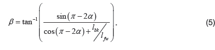
The slope angle
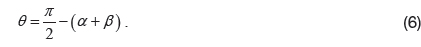
In the above figure,
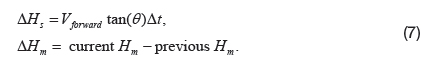
Finally, the height variation of the vehicle is computed as

3.3 Integrated Navigation Filter
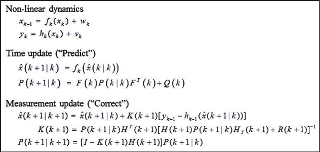
There are various filtering methods, such as the EKF, UKF (unscented Kalman filter), CKF (cubature Kalman filter), and PF (particle filter) for nonlinear system application. In many cases, the EKF approach for the nonlinear estimation problem provides a strong cost-effective result, in comparison with other nonlinear estimation methods. Thus in this paper, considering aspects of algorithm complexity, estimation performance, and onboard hardware implementation, the integrated navigation filter is constructed based on the EKF framework, using the INS error model and sensor measurement models in the previous sections. In this scheme, the linearized system and observation model around the last state estimates are used for each time update, and measurement update computation. Fig. 4 briefly summarizes the formulations of the EKF.
The state vector consists of position, velocity and attitude error of the vehicle; and additionally, bias errors of the IMU measurements are augmented. The state can be expressed as

The dynamics of the system model has the following form. Detailed expression for the dynamic matrix, F is shown in Appendix A.

where,
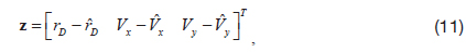
The observation vector consists of the altitude difference between the altitude estimated from the INS and LiDAR altitude, and horizontal velocity difference with respect to the body frame, between velocity estimated from the INS, and that calculated using optical flow vectors. Thus, the observation vector can be expressed as

where,
rD : Vertical position w.r.t the navigation frame(NED frame) : Computed vertical position w.r.t. the navigation frame, using LiDAR measurements : Computed horizontal velocity, using optical flow vectors.
The observation model, representing relations between the state vector and the observation vector, is modeled as (12).

The measurement matrix is represented by
where, : Transformation matrix from the navigation frame to body frame. In the above models, all process and measurement noises are modeled as zero-mean white gaussian noises.
Fig. 5 represents the structure of the proposed integrated navigation filter. An indirect feedback structure is adopted, to compensate estimated error. In this filter structure, the integrated navigation solution is estimated by compensating the estimated INS error, using the measurement vectors from optical flow and LiDAR.
The feasibility of the proposed integrated navigation filter in the previous section was verified through simulations, by comparing the navigation performance of the proposed system, with that of an INS-only system, when GNSS signal outage occurs.
The navigation scenario is that a fixed-wing UAV first makes a level flight with GNSS/INS navigation mode, and then the navigation mode is changed to an integrated navigation system, as soon as GNSS signal outage occurs, at 10 seconds from the beginning. After that, the vehicle navigates with integrated navigation mode to the end. In this process, it is assumed that detecting whether GNSS signal can be used or not, and switching navigation node, are accomplished by another algorithm. The detailed flight profile is shown in Table 1.
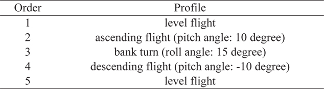
Flight profile
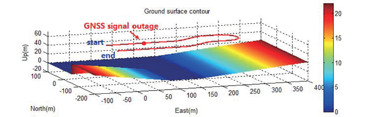
The ground surface has a slope angle of 5 degrees, after 150 meters in an easterly direction, and -7 degrees between -100 meters and 80 meters in an easterly direction, at the end of the trajectory of the vehicle, as shown in Fig. 6. When generating height distribution, the horizontal position resolution is set to 0.1 meters.
The total simulation time is set to 75 seconds, and during the beginning 10 seconds, an initial alignment process is conducted, to calculate the initial attitude, and estimate biases of the IMU measurements. GNSS signal outage occurs from 10 seconds after the vehicle starts moving, to the end. In this process, bias values and the covariance matrix that are estimated just before the GNSS signal blockage occurs are used as the initial bias values and covariance matrix in the proposed system. The IMU operates at 100Hz, and the vision sensor and LiDAR provide their measurements at 5Hz. Specifications of the sensors are presented in Table 2 below.
[Table 2.] Sensor data specification
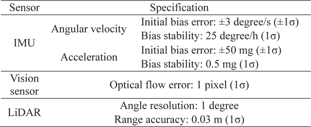
Sensor data specification
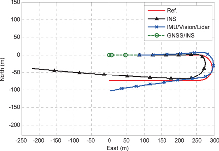
In the simulation, the initial alignment is done in advance, to generate the initial bias and covariance estimate value. Fig. 7 shows the horizontal position estimate results. In the case of the INS only system, the error of the estimate gradually increases and diverges as time goes on, after the GNSS signal outage occurs. In particular, the error in an easterly direction is beyond 200 meters. On the other hand, the IMU/Vision/ Lidar integrated system tracks the reference trajectory well, and its divergent characteristic becomes much weaker than the other. This is because the optical flow vectors and LiDAR measurements are utilized, for estimating the INS errors in the integrated navigation filter.
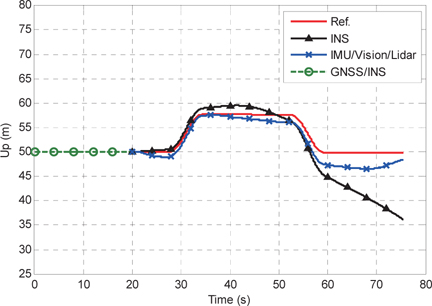
The altitude estimate results are very similar to the horizontal position estimate results. Fig. 8 shows the vertical position estimate results. In this graph, the INS error diverges, as time goes on; whereas the integrated system shows reliable estimation performance. Despite its good estimation performance, the estimation error grows slightly during short intervals of around 25 sec and 60 sec, where the error in range measurement increases notably. This occurs when the LiDAR heads the intersection regions, in which the flat surface and sloping surface coexist at around 25 sec, and the flat surface and two sloping surfaces coexist at around 60 sec. Measurement errors are relatively amplified, as the angle between the sloping surface and the LiDAR measurements gets smaller. Furthermore, the horizontal position resolution, when generating the height distribution of the ground surface, is correspondingly degraded.
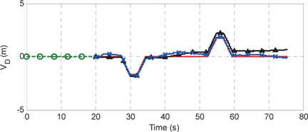
Fig. 9 shows the velocity estimate results. In common with the position estimate results, the performance of the integrated system is better than that of the INS only system.
Quantitative error analysis of the estimated position/ velocity is presented in Table 3. Root mean square errors (RMSE) of the estimated position/velocity are calculated, using the simulated true values.
[Table 3.] Error analysis of the estimated position and velocity
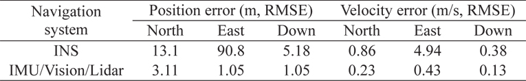
Error analysis of the estimated position and velocity
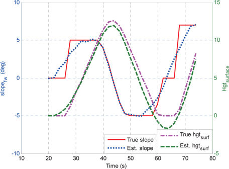
Fig. 10 shows estimate results of the slope angle and height of the ground surface. The estimated slope angle is not the slope angle of the real ground surface, but that of the virtual ground surface. Thus, in the intersection areas, the estimated slope is different from the true slope. Also, the characteristic of the altitude measurement model is reflected in the estimation result of the height of ground surface. In this graph, the error of the estimated height of the ground surface becomes slightly larger, since the LiDAR measurement error and the error of the estimated forward velocity affect height variation of the ground surface.
In this simulation, the integrated filter cannot estimate all state variables, due to the limitation of the flight maneuvers, which can affect the observability of the system. The proposed system can be modeled as PWCS (Piece-Wise Constant Systems), and their observability can be analyzed by SOM (Stripped Observability Matrix) rank analysis. Since observable state variables and their linear combinations are determined according to the maneuvering mode of a vehicle, the proposed system can be a fully observable system, when longitudinal and lateral acceleration are applied to the system. Verification of this theoretical analysis result can be further investigated, via more advanced simulations and experiments.
In this paper, we proposed a Vision/LiDAR aided integrated navigation system, in the limited environments in which GNSS signals cannot be used, the height of the ground surface is varying and there is no map information. The proposed system consists of a MEMS IMU, a vision sensor and a LiDAR. In this system, the IMU is mounted on the vehicle body, and the vision sensor and LiDAR are mounted on a two-dimensional gimbal system, in order that those sensors always maintain the horizontality condition. The proposed system can provide reliable navigation solutions, by suppressing rapid divergence of the INS error, using vision sensor and LiDAR measurements. The horizontal velocity estimate of the INS is corrected, by using optical flow measurements from the vision sensor, and range information between the system and the ground surface, from LiDAR. At the same time, the height of the ground surface is estimated, by using forward/backward LiDAR measurements; therefore, with the estimated height, the accurate altitude can be obtained. For these purposes, an integrated navigation filter is constructed, based on the EKF framework. The feasibility of the system is proved via simulation results.
In the simulation, the performance of the proposed integrated navigation system was verified, by comparing the navigation performance of the proposed system, with that of the INS only system when GNSS signals cannot be used. As a result, our proposed integrated system provides more accurate navigation solutions than the INS. However, the problem that position error slowly increases still remains, because the system navigates relatively, without absolute navigation information, such as GNSS signals, landmarks, and so on. This problem is regarded as an inevitable limitation of a standalone navigation system.
The integrated navigation system proposed in this paper is expected to be applicable to various fields that require relative navigation information, such as a low altitude UAV that operates in the downtown area, or jamming environments, in which the GNSS availability is low.


![Summary of the EKF formulations [20]](http://oak.go.kr/repository/journal/13491/HGJHC0_2013_v14n4_369_f004.jpg)