


The in-depth understanding of aeroelastic effects on deformable lifting bodies (LBs), due to steady and unsteady aerodynamic loadings, is a typical challenging issue for the current design of aerospace vehicles [1]. Furthermore, with the forthcoming employment of composite materials in next-generation aircraft configurations, such as High-Altitude Long Endurance aircraft (HALE) [2], and strut-braced wings [3], accurate evaluation of the aeroelastic response becomes even more crucial [4].
Recently, special attention has been directed to the profitable exploitation of the aeroelastic phenomena comprehension , by studying the concept of morphing wings, which are able to adapt and optimize their shape depending on the specific flight conditions and mission profiles [5, 6]. The smart wing is very flexible and could allow a number of advantages, such as drag reduction and aeroelastic vibrations suppression by means of adaptive control [7] and different solutions, such as compliant structures [8], bi-stable laminate composites [9], piezoelectric [10] and shape memory alloy actuation [11].
In order to develop aeroelastic tools that are able to work in any regime and with any LB geometry, the literature from the last decades has been widely influenced by research devoted to build reliable methods, to couple computational fluid dynamics (CFD) or classical aerodynamic methods with the finite element method (FEM) for structural modeling [12]. Valuable examples are in the review articles by Dowell and Hall [13], and Henshaw et al. [14]. Reduced approaches, for instance panel methods, are widely used for the classical aerodynamics of wings under some limitations [15], allowing a sizeable reduction in terms of computational cost [16,17]. The assumption of undeformable airfoil-crosssections [18] is typically not proper for recent configurations, since the weight reduction makes wings more flexible and highly-deformable. Hence, two-dimensional (2D) plate/shell and three-dimensional (3D) solid methods are usually employed for the structural modeling, instead of classical one-dimensional (1D) theories, such as the Euler-Bernoulli, Timoshenko, or Vlasov theories [19].
With the advent of smart wings, detailed structural and aeroelastic models are even more essential to fully exploit the non-classical effects in wing design, due to the properties characterizing advanced composite materials, such as anisotropy, heterogeneity and transverse shear flexibility. Beam-like components can be analyzed by means of refined one-dimensional (1D) formulations, which have the main advantage of a lower computational cost required compared with 2D and 3D models. A detailed review of the recent development of refined beam models can be found in [20]. El Fatmi [21] improved the displacement field over the beam cross-section, by introducing a warping function, to refine the description of normal and shear stress of the beam. Generalized beam theories (GBT) originated with Schardt’s work [22] and improved classical theories, by using a piecewise beam description of thin-walled sections [23]. An asymptotic type expansion, in conjunction with variational methods, was proposed by Berdichevsky et al. [24], where a commendable review of prior works on beam theory development was given. An alternative approach to formulating refined beam theories, based on asymptotic variational methods (VABS), has led to an extensive contribution in the last few years [25].
A considerable amount of research activity devoted to aeroelastic analysis and optimization was undertaken in the last decades, by using reduced 1D models. A review was carried out by Patil [26], who investigated the variation of aeroelastic critical speeds with the composite ply lay-up of box beams, via the unsteady Theodorsen’s theory. A thin-walled anisotropic beam model in-corporating non-classical effects was introduced by Librescu and Song [27] to analyze the sub-critical static aeroelastic response, and the divergence instability of swept-forward wing structures. Qin and Librescu [28] developed an aeroelastic model to investigate the influence of the directionality property of composite materials, and non-classical effects on the aeroelastic instability of thin-walled aircraft wings. Among the several composite rotor blades applications, the work done by Jeon and Lee [29] concerning the steady equilibrium deflections, via a large deflection type beam theory with small strains, is worth mentioning. An example of the use of a refined beam theory for aeroelastic analysis can be found in [30], where the static and dynamic responses of a helicopter rotor blade are evaluated by means of a YF/VABS model.
Higher-order 1D models with generalized displacement variables, based on the Carrera Unified Formulation, have recently been proposed by Carrera and co-authors, for the static and dynamic analysis of isotropic and composite structures [31]. The CUF is a hierarchical formulation, which considers the order of the model as a free-parameter of the analysis. In other words, models of any order can be obtained, with no need for ad hoc formulations, by exploiting a systematic procedure. Structural 1D CUF models were used to analyze the structural response of isotropic aircraft wings, under aerodynamic loads computed through the Vortex Lattice Method (VLM), in [32]. The aeroelastic CUF-VLM coupling was preliminarily formulated in [33] for isotropic flat plates, and then extended to instability divergence detection and the evaluation of composite material lay-up effects on the aeroelastic response of moderate and high-aspect ratio wing configurations, in [34]. Flutter analyses of composite lifting surfaces were also presented in [35], by coupling the CUF approach with the Doublet Lattice Method.
The present work couples a refined one-dimensional finite element model based on CUF to an aerodynamic 3D Panel Method, implemented in the software XFLR5. Two potential methods are here compared: the VLM and the 3D Panel Method. The aeroelastic static response of a straight wing is computed through a coupled iterative procedure, and a linear coupling approach. Particular attention is drawn to the in-plane deformation of the wing airfoil cross-sections, as well as the aeroelastic influence of free stream velocity.
2. Numerical models: refined 1D CUF model and panel methods
2.1 Variable kinematic 1D CUF FE model
For the sake of completeness, some details about the formulation of CUF finite elements are here retrieved from previous works [32, 34]. A structure with axial length

where

The variational statement employed is the Principle of Virtual Displacements:

where

where

Using Eq. 5, Eq. 3 can be rewritten in terms of virtual nodal displacements:

where, the 3 × 3 and 3 × 1

where is the structural stiffness matrix, and is the vector of equivalent nodal forces. It should be noted that no assumptions on the expansion order have so far been made. Therefore, it is possible to obtain higher-order 1D models without changing the formal expression of the nuclei components, as well as classical beam models, such as Euler-Bernoulli’s and Timoshenko’s. Higher-order models provide an accurate description of the shear mechanics, the in-plane and out-of-plane cross-section deformation, Poisson’s effect along the spatial directions, and the torsional mechanics, in more detail than classical models do. Thanks to the CUF, the present hierarchical approach is invariant with respect to the order of the displacement field expansion. More details are not reported here, but can be found in the work of [31].
2.2 A numerical approach for wing aerodynamic analysis
The evaluation of aerodynamic loads can be typically carried out through a CFD code, which solves, for example, either Navier-Stokes equations or Euler equations numerically. This kind of analysis has a high computational cost, but under some assumptions it is possible to employ simplified approaches. In the wing cases considered in the present work, the flow field is assumed to be steady, and the fluid viscosity is not decisive since the viscous effects can be confined into a small region (boundary layers and wake regions). The fluid can be thus considered as inviscid, and the flow is irrotational, since the curl of the velocity vector (

In this case, the velocity vector (

Hence, the analysis of a wing or an airfoil under these conjectures can be performed by potential methods. The potential function describing the flow field around an object can be defined as a combination of singularities, such as doublets, vortices, sources, or uniform flux over the external body surface. According to the detailed exposition in [36], the equation to be used to compute the solution of the aerodynamic problem is Laplace’s equation:

Laplace’s equation describes a potential flow field only if the compressibility effects can be neglected, as occurs for the results presented afterwards, where the free stream velocity is rather low. Otherwise, some corrections, e.g. the Prandtl-Glauert transformation, are necessary, as explained in [37]. The assumptions here introduced lead to an integral-differential equation, which expresses the potential function in an arbitrary point of the fluid domain as a combination of singularities. For the sake of brevity, this equation is not reported here, but more details can be found in [36]. Among the potential methods, the panel methods can be formulated following a low-order, or a high-order approach. The loworder (first-order) panel method employs triangular or quadrilateral panels having constant values of singularities’ strength, such as the Hess and Smith approach. The higherorder panel methods instead use higher than first-order panels (e.g. paraboloidal panels) and a varying singularity strength over each panel.
2.2.2 XFLR5: an implementation of aerodynamic potential methods
XFLR5 is a software developed by Andre Deperrois. It performs viscous and inviscid aerodynamic analysis on airfoils and wings using three potential methods: the Lifting Line Theory (LLT), the VLM and the 3D Panel Method. The LLT method derives from Prandtl’s wing theory and considers the wing as a linear distribution of vortices. The VLM considers a wing as an infinitely thin lifting surface, via a distribution of vortices placed over a wing reference surface. This method requires the non-penetration condition on the reference surface as a boundary condition. Hence, the normal component of the induced velocity on the generic

Further details on this method can be found in [15]. The 3D Panel Method schematizes the wing surface as a distribution of doublets and sources. The strength of the doublets and sources is calculated to meet the appropriate boundary conditions (BCs), which may be of Dirichlet- or Neumann-type. According to the creator of the program, after a trial and error process, the best results can be obtained by using just the Dirichlet BC type [38]. The 3D Panel Method employs a low-order panel method. The LLT approach is not able to evaluate the pressure coefficients on the wing surface, but only the lifting loads along the lifting line. The VLM is able to analyze the pressure coefficients, but only on the reference surface, which is defined as the mean surface between the upper and the lower wing surfaces. The 3D Panel Method is able to calculate the pressure coefficients on both the upper and the lower wing surfaces. Therefore, this method offers the most realistic description of the aerodynamic field.
3. Aeroelastic static response analysis via the CUF-XFLR5 approach
In this work the aeroelastic static response of the wing is computed through an iterative procedure, based on a coupled CUF-XFLR5 method. Hence, the aerodynamic analysis is performed through the potential methods available in XFLR5, as previously mentioned; whereas, variable kinematic 1D CUF models provide the structural wing deformation with a variable expansion order
Figure 1 shows in detail the aeroelastic iterative process, which starts with the evaluation of the pressure coefficients for the undeformed wing configuration. The further steps to be repeated for each iteration are:
1. post-processing calculation of the aerodynamic forces; 2. structural analysis of the wing subject to the aerodynamic forces previously computed; 3. new calculation of the aerodynamic pressure coefficients for the new deformed configuration; 4. post-processing evaluation of the wing deformation and cross-section distortion.
Structural displacements are evaluated in specific sections distributed regularly along the wing span. The cross-section distortion

where △
The iterative process in Fig. 1 is stopped once the convergences of the lifting coefficient


where
3.2 Aerodynamic loads computation
The aerodynamic load computed by XFLR5 is a distributed pressure and in this work it is modeled as distributed forces. The generic force acting on the j-th aerodynamic panel is evaluated as:

where
For each iteration, the three-dimensional deformed configuration of the wing is built using 11 airfoils along the half-wing span, at a distance of 0.5 m from each other. The first section lies at the wing root. The wing is discretized through a lattice of quadrilateral aerodynamic panels. Let be the number of panels along the chord line and let be the number of panels along the half-wing span. When the VLM is employed the total number of aerodynamic panels
Firstly, an aerodynamic assessment of the VLM and the 3D Panel Method, which are able to evaluate the pressure coefficients on the wing surface, is performed analyzing the effects of two typical geometrical parameters: the airfoil thickness and the camber line. A straight wing is considered: the wing span is 10 m, and the airfoil chord is 1 m long, as drawn in Fig. 2a, where the right half-wing is depicted. This wing configuration is also used in the following structural and aeroelastic analyses. The effect of the camber line on the aerodynamic field is evaluated, using NACA 2415, 3415 and 4415 airfoils. The analysis of the influence of the airfoil thickness is then carried out, using the symmetric NACA 0005, 0010 and 0015 airfoils. The number of aerodynamic panels is chosen as a compromise between the limit number of panels that can be used in XFLR5 (= 5,000) [38], and the number of panels required, in order to achieve convergence in the aerodynamic results. In the following analyses, the choice of = 24 and = 50 remains the same.
For the present assessment analysis, the free stream velocity is assumed to be

where,
Figure 3b reports the trend of the spanwise local lifting coefficient
In order to validate the results given by the proposed higher-order 1D CUF approach, a comparison of the static structural wing response is here performed, with MSC Nastran. Only the right half-wing of the straight configuration introduced in the previous aerodynamic assessment (see Fig. 2a) is considered here, due to loads and structural symmetry. A clamped boundary condition is taken into account for the root cross-section (at
Due to the small thickness and the well-known aspect ratio restrictions typical of solid elements, this wing is modeled in MSC Nastran by 214,500 solid Hex8 elements and 426,852 nodes, corresponding to 1,280,556 degrees of freedom (DOFs). The same structure is analyzed through CUF models with a variable expansion order up to
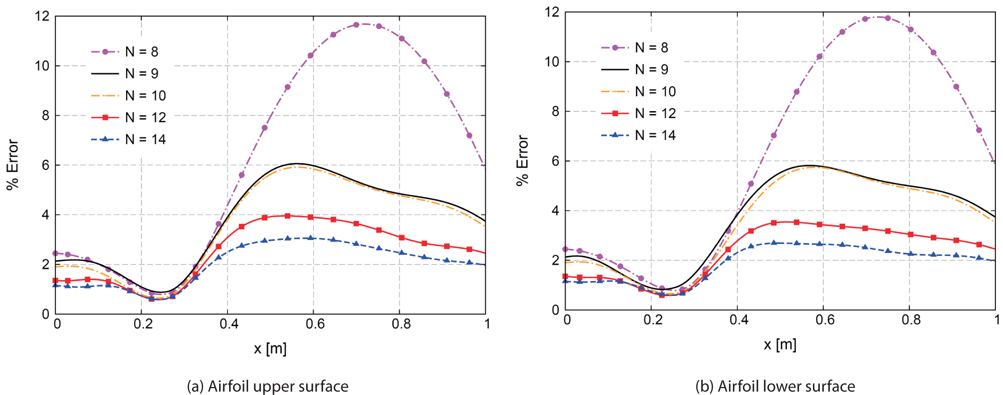
A variable pressure distribution step-like along the spanwise direction is applied to the upper and lower wing surfaces, in order to simulate a real pressure distribution, see Table 1. The static structural response of the wing is evaluated in terms of the distortion s at the tip cross-section. For the upper and lower surfaces, Figs. 4a and 4b show the percent error


Pressure distribution on the wing along the spanwise direction, for the structural assessment. V∞=50m/s, ρ∞=1.225kg/m3
As depicted in Figs. 4a and 4b, the proposed 1D FEs provide a convergent solution, by gradually approaching the Nastran solid results, as the expansion order increases from 8 to 14, according to the conclusions made in previous CUF works [39]. For
This section focuses on the results regarding the equilibrium aeroelastic response of a wing exposed to a free stream velocity
The 1D structural mesh consists of 10 B4 elements. For the sake of brevity, a convergent study on the number of mesh elements is not reported here. In fact, the choice of 10 B4 elements yields a good evaluation of displacements for all the points of the structure, as detailed in [32,34], where a similar structural case in terms of wing configuration and applied aerodynamic loads was studied via the present structural model, and successfully assessed with a commercial FE solid model.
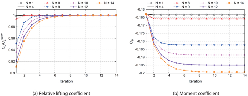
The aeroelastic analysis is now carried out following the iterative coupled procedure CUF-XFLR5 described in Fig. 1 and varying

Convergent values of lifting coefficient and moment coefficient for different structural models. V∞ = 30 m/s, =0.4637, =-0.1629.
Hence, a different choice of
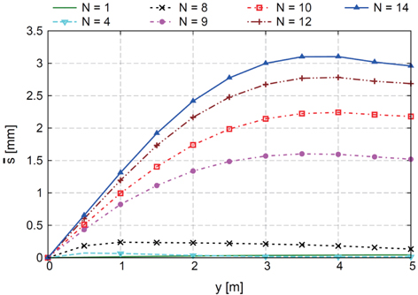
An average cross-section distortion is now introduced in order to evaluate the aeroelastic deformation of the cross-section shape along the wing span. Given an airfoil cross-section, the average distortion is defined as:

where
For this cross-section, Table 3 presents the numerical values of average distortion in the iterative aeroelastic analysis for different structural theories. As occurred for the convergence of aerodynamic coefficients, the number of iterations required to achieve the convergence of increases as

Convergence of the average distortion [mm] in the iterative aeroelastic analysis, for different structural models. Airfoil cross-section at y=4m. V∞=30m/s.
For
As expected, low-order models provide a correct evaluation of the bending and torsional structural behavior, but not an exhaustive description of the in-plane deformation. This conclusion is confirmed by Fig. 8, where the airfoil distortion

Convergent average distortion [mm] of the cross-section at y=4m for different structural models. Values and chordwise positions of the maximum distortions [mm] and [mm] on airfoil upper and lower surfaces. V∞= 30 m/s.
In general, improvements of the structural theory yield more realistic deformations of the wing, until a good convergence is achieved for
4.4 Free stream velocity influence
This analysis aims at establishing the influence of the free stream velocity on the wing distortion. The wing configuration employed for this analysis is the same as that used in the previous study. According to the previous conclusion, the structural model considered is
In this case, and represent the final convergent values of the lifting and moment coefficients for a given
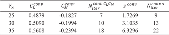
Convergent values of lifting coefficient , moment coefficient ,and average distortion [mm] of cross-section at y=4m, for different free stream velocities V∞ [m/s]. Structural model: N=14. =0.4637, =-0.1629.
The limitation of distortion close to the airfoil leading edge due to the spar is enhanced for

Values and chordwise positions of the maximum distortions , , , [mm] on the airfoil upper and lower surfaces of the cross-section at y=4m, for different free stream velocities V∞[m/s]. Structural model: N=14.
Variable kinematic 1D finite elements were formulated on the basis of Carrera Unified Formulation (CUF) and coupled to an aerodynamic 3D panel method implemented in XFLR5. The aeroelastic static response of a straight wing with a highly-deformable airfoil cross-section was computed through a coupled iterative procedure, for an increasing structural accuracy and for different free stream velocities. An aerodynamic assessment confirmed that the 3D Panel Method provides a more realistic evaluation of the pressure distribution on the wing, than the Vortex Lattice Method (VLM). As far as the use of 1D higher-order models is concerned, the following main conclusions can be drawn:
1. The introduction of higher-order terms in the displacement field is even more important for the aeroelastic analysis, due to the fluid-structure coupling. 2. In the case that the wing is rather flexible, the in-plane cross-section deformation has a great impact on the alteration of the aerodvnamic loadings. 3. The higher the free stream velocity, the more marked the in-plane distortion effect.
As far as the present hierarchical one-dimensional approach is concerned, the results point out that:
a. The CUF is an ideal tool to easily compare different higher-order theories, since the model accuracy is a free parameter of the analysis. The in-plane airfoil cross-section deformation is well-described by the proposed 1D structural model, in good agreement with a three-dimensional FE solution, and with a remarkable reduction in terms of DOFs. c. A convergent trend of displacements and aerodynamic coefficients is achieved as the structural model accuracy increases. This proves that the proposed 1D higher-order approach does not introduce additional numerical problems in the aeroelastic analysis of wings with arbitrary cross-section geometry. d. A higher number of iterations is necessary to achieve convergence on structural distortion than for convergence on aerodynamic coefficients.
These reasons make the future use of the proposed CUF-XFLR5 approach appear promising for a versatile flight optimization tool.


![Convergence of the average distortion [mm] in the iterative aeroelastic analysis, for different structural models. Airfoil cross-section at y=4m. V∞=30m/s.](http://oak.go.kr/repository/journal/13487/HGJHC0_2013_v14n4_310_t003.jpg)


![Convergent average distortion [mm] of the cross-section at y=4m for different structural models. Values and chordwise positions of the maximum distortions [mm] and [mm] on airfoil upper and lower surfaces. V∞= 30 m/s.](http://oak.go.kr/repository/journal/13487/HGJHC0_2013_v14n4_310_t004.jpg)

![Convergent values of lifting coefficient , moment coefficient ,and average distortion [mm] of cross-section at y=4m, for different free stream velocities V∞ [m/s]. Structural model: N=14. =0.4637, =-0.1629.](http://oak.go.kr/repository/journal/13487/HGJHC0_2013_v14n4_310_t005.jpg)


![Values and chordwise positions of the maximum distortions , , , [mm] on the airfoil upper and lower surfaces of the cross-section at y=4m, for different free stream velocities V∞[m/s]. Structural model: N=14.](http://oak.go.kr/repository/journal/13487/HGJHC0_2013_v14n4_310_t006.jpg)


