The Discrete Fourier Transform (DFT) method is widely used in harmonic measurements of industrial power systems [1-3], which are steady and dependable, and can be easily implemented in embedded systems. In addition, the DFT based method has been adopted by the IEC61000-4-7 standard [4]. However, the DFT method is subject to errors from an effect known as spectral leakage [5,6]. This effect occurs when the DFT is computed from a block of data that is not periodic. In practice, weighting samples by different windows is one of the main approaches to suppress error caused by spectral leakage [7-10]. The windowing can be easily handled in the frequency-domain. Choosing an appropriate window can significantly depress the discontinuity caused by incoherent sampling. Up to now, various window functions have been proposed and used for harmonic analysis, including Hanning window [11], Hamming window [7], Blackman window [7], Blackman-Harris window [12], Nuttall window [8], Rife- Vincent window [13], flat-top window [14] and self-convolution window [15-18], among others. Each type of window affects the spectrum in a slightly different way and has its own advantage and disadvantage relative to the others.
The main problem that the Windowed DFT suffers from is synchronous deviation, random noise and inter-harmonics. In fact, initial-phase sensitivity should also be considered. For years many studies have concentrated on synchronous deviation [7,19,20], random noise [21-23], and inter-harmonics [24,25], however there is a lack of knowledge about initial-phase sensitivity [26]. Initial-phase sensitivity is the influence to amplitude accuracy, which is caused by the randomness of the initial-sampling phase. The initial-sampling phase corresponds to the starting position of time series. In practical engineering, the sampling of the signal is random [27,28], that is, the initialsampling instant is stochastic. Therefore it is difficult to ensure that the initial-sampling phase is identical every time. Randomness of initial-sampling phase leads to a variety of spectral leakage, resulting in instability of measurement, especially for weak-frequency components. According to IEC 61000-4-7 [4], harmonic measurement instrument should be able to analyze weak harmonic, accordingly it is important to study the problem of initial-phase sensitivity. There is a close relationship between harmonic amplitude and the initial-sampling phase mentioned in [29]. However, further research has not been carried out to study the effect of initial-sampling phase on amplitude accuracy.
In this paper, the origin of initial-phase sensitivity has been analyzed in theory, and then the major factors that affect the level of initial-phase sensitivity have been studied. In addition, the method has been put forward to reduce initial-phase sensitivity.
2. INITIAL-PHASE SENSITIVITY STUDY
2.1 Theoretical analysis of initial-phase sensitivity
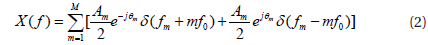
Assuming that the periodic signal x(t) with fundamental frequency fo is composed of M tones as follows:
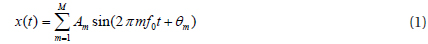
Am, θm are the amplitude and phase of the mth harmonics. The Fourier transform of x(t) can be written as follows:

Assuming that w(t) is an arbitrary continuous window function well-defined in [-L/2, L/2] intervals, additionally the window function is symmetrical, e.g. Blackman window, Hanning window. L is the length of the window. The Fourier transform of w(t) is obtained

As there is no negative time, in the case where the time starts at zero at the beginning of sampling, when the finite discrete sequence of w(t) is processed by the Fourier transform, the real windowing intervals is [0, L], that is, window function is shifted half the length of the window in the time axis. The shifted window function is marked as wL(t). According to the time shift characteristic of Fourier transforms, the Fourier transform of wL(t) is

After x(t) is multiplied by the window function wL(t), based on the frequency-domain convolution theorem the Fourier transform of x(t)wL(t) is
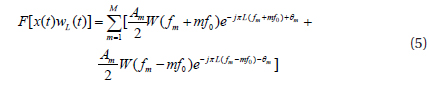
For a periodic signal and arbitrary window function, equation (5) always holds. According to equation (5), the spectral characteristics of F[x(t)wL(t)] are determined by function W(f).
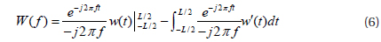
The subsection integral of equation (3) can be expressed as follows:

Since the value of is zero at the boundary of the scope, then the first term is zero in equation (6). As function w(t) is composed of elementary functions, it is impossible for the infinite order derivative of w(t) to be smooth, otherwise w(t) would always be zero. Accordingly it is certain that there is a positive integer K, which make w(k)(t) non-differentiable, and then w(k)(t) must be a piecewise continuous function. As to window functions, the discontinuous points of w(k)(t) are at the ends(t=±L/2), so the derivative order of w(t) is K-1, and satisfies w(k)(L/2)=w(k)(-L/2)=0 (k=0, 1, ..., K-1).
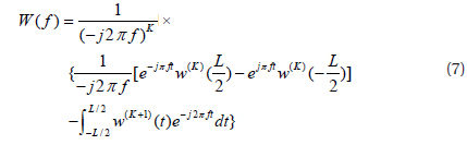
Integration by parts is performed on equation (6) again and again, in this way equation (7) is obtained

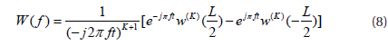
On the condition that |f|→∞, in equation (7), the integral term in braces trends to zero. So, equation (7) can be expressed as follows:

In equation (8), there are two oscillating functions with a frequency of ±4 π/L. The combination of the two oscillating functions is still an oscillating function, and the frequency of the combined function remains unchanged. The decay speed of W(f) is determined by 1/(−j2 πft)k+1. Therefore, W(f) is always in a state of oscillation and attenuation, and it is impossible to eliminate the oscillation (side lobe) by choosing the shape of the window function. Therefore, DFT windows reduce the effects of spectral leakage but cannot eliminate leakage entirely.
In the synchronous case, there is no mutual interference between the harmonic components, in addition harmonic components fall at frequencies that are integer multiples, consequently the estimation of signal is very accurate based on windowed DFT. Nevertheless, it is difficult to realize strictly synchronous sampling because the system's fundamental frequency usually deviates from its nominal value of 50/60 Hz, which is caused by the power system load and generation variations [30]. Even if the approach of synchronizing software/hardware is applied for sampling, which just provides the frequency of the last period, the frequency of the current period still cannot be confirmed accurately.
In the non-synchronous case, the form of equation (5) can be written as follows:
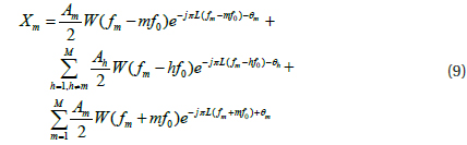
In equation (9), the first term denotes the complex spectrum of the mth harmonics, and its actual frequency fm deviates from the normal frequency mfo. The second and the third terms represent the complex spectrum of other harmonics at fm except the mth harmonics, including the complex spectrums generated by negative frequencies.
Due to the randomness of initial-sampling, different starting positions of the time series corresponds to different initial phases of the respective harmonic components. In equation (9), the change of initial phase of the second and the third terms leads to the change of spectral value itself, this then influences the value of Xm. This changed Xm results in the variation of harmonic amplitude.
Accordingly, in the non-synchronous case, the randomness of the initial-sampling gives rise to the change of spectral leakage, and then has an effect on the amplitude accuracy. This problem is initial-phase sensitivity.
To demonstrate the existence of initial-phase sensitivity, several simulations were carried out by MATLAB. The current/ voltage signals in power systems mainly include fundamental frequency component and harmonics. Since the spectrum of the cosine window functions is equally spaced, the algorithm based on cosine-windowed DFT is commonly selected for harmonic measurements. In this paper, the combined cosine window functions mentioned in [7] are selected for simulation, these include Hanning window, Hamming window, Blackman window and 4-term Blackman-Harris window.
Here the signal model of current in [26] is chosen for simulation. The harmonic signal is
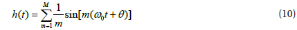
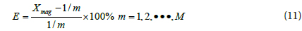
Where 𝜔0, θ, denote the angular frequency and initial phase of the power fundamental harmonic; the highest order of harmonic M=50; the fundamental frequency is 50 Hz; the relative synchronous deviation is 1%. The accurate period of the signal is 2 π (in radians). The sampling points per cycle are 128, which is expressed by P; the sampling time unit is τ=1.01×2 π/P. In order to describe initial-phase sensitivity, the concept of relative error of amplitude is introduced, represented by the capital letter E. The equation of relative error of amplitude is

In equation (11), 1/m is the real amplitude of the mth harmonic, and Xmag denotes the calculated amplitude of the mth harmonic.
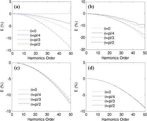
During the course of the simulation, all the time record lengths used for windowed DFT are adopted with the least analysis periods. For example, the least test period of Hanning-windowed DFT is two periods of the fundamental component. Fig. 1 shows the simulation results, illustrating the relative errors of amplitude when the initial phase equals 0, π/4, π/3, π/2 (in radians) respectively. For Fig. 1(a) to Fig. 1(d), the window function used for simulation is Hanning window, Hamming window, Blackman window and 4-term Blackman-Harris window, respectively.
The simulation results, shown in Fig. 1, indicate the interference from the randomness of initial-sampling phase on amplitude accuracy. The maximum relative error of amplitude caused by initial-phase sensitivity are 17.66%, 12.29%, 1.06% and 0.15% respectively for the four types of window function applied
On the basis of the simulation above, it is confirmed that initial-phase sensitivity really has an effect on amplitude accuracy, especially for weak harmonics, but it should not always be considered. When Hanning window and Hamming window are applied, initial-phase sensitivity should be considered; however initial-phase sensitivity can be neglected if the Blackman window and 4-term Blackman-Harris window are adopted. Thus when window functions are chosen for harmonic analysis, initial- phase sensitivity should be considered for certain windows or not included for others.
3. FACTORS AFFECTING THE INITIALPHASE SENSITIVITY
Since not all the windows used for harmonic analysis should consider initial-phase sensitivity, to enhance the stability of windowed DFT it is necessary to study the factors that affect the level of initial-phase sensitivity, and also find the constraints that do not need to consider initial-phase sensitivity.
3.1 Major factors influencing the initial-phase sensitivity
Spectral leakage is closely related to synchronous deviation of sampling and side lobe characteristics of the window function [7,15], and the effect of initial-phase sensitivity makes the level of spectral leakage changeable within certain scopes, thus initialphase sensitivity must be bound up with synchronous deviation and side-lobe characteristics of the window. So when synchronous deviation is certain, initial-phase sensitivity is decided by the side-lobe characteristics of the window. The side-lobe characteristics of the windows that are applied for simulation in Section 2 are shown in Table 1.
[Table 1.] Side lobe characteristics of classical cosine window.
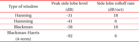
Side lobe characteristics of classical cosine window.
Comparing Fig. 1 with Table 1, we can see that initial-phase sensitivity decreases with a decrease of the peak side lobe, from Hanning window, Hamming window, Blackman window to Blackman-Harris window. Meanwhile the side lobe rolloff rate of these windows has not direct influenced the initial-phase sensitivity. For example, although the side lobe rolloff of the Hanning window is larger than that of the Hamming window, initial-phase sensitivity is smaller. Thus, according to the simulation in section 2 and the side lobe characteristics of the same windows in Table 1, the initial-phase sensitivity is determined by the peak side lobe level of the window: the lower the peak of the side lobe level of the window, the smaller the initial-phase sensitivity.
In order to verify whether initial-phase sensitivity is decided by the peak side lobe level of the window, when synchronous deviation of sampling is certain, Kaiser window is introduced. By using the feature that the parameter of Kaiser window can be modified freely, choosing the peak side lobe level of Kaiser window is equivalent to the peak side lobe level of one of the windows that are used for simulation in section 2, meanwhile the side lobe rolloff rate for the two windows is different. In this case, the initial-phase sensitivity is identical, thus it is confirmed that initial-phase sensitivity is decided by the peak side lobe level of the window. In this paper, Blackman window is chosen to compare with Kaiser window (β=8, β is the adjustable parameter of Kaiser window). The peak side lobe level of the two window functions is identical (−58 dB) and the side lobe rolloff rate is different (the side lobe rolloff rate of Blackman window is 18dB/oct, and that of Kaiser window (β=8) is 12 dB/oct).
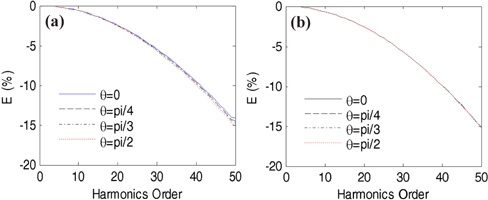
The procedures for verification are as follows: first, Blackman window and Kaiser window(β=8) are used for the signal analysis in equation(10) based on windowed DFT, and the initial phase of the harmonics is 0, π/4 (in radians, of course other initial phases can be selected freely). Second, two groups of amplitudes are achieved under the same window function, and subtraction is conducted between the two groups of amplitude, and then the same behaviors are repeated for the other window function. Third, a comparison is performed between the differences of the two groups of amplitude. If the differences of the two groups of the amplitudes are identical, the fact that the initial-phase sensitivity is decided by the peak side lobe level of window is confirmed.
A comparison of the amplitude difference between Blackman window and Kaiser window(β=8) is shown in Fig. 2. The plots in Fig. 2 show that two groups of amplitude difference are almost coincident, except that there is a slight diversity before the nineteenth harmonic. Accordingly, under the condition that synchronous deviation of sampling is certain, the error of the amplitude that is introduced by the initial-phase sensitivity has nothing to do with the side lobe rolloff rate of the window, and initial-phase sensitivity is decided by the peak side lobe level of window.
In addition, when the peak side lobe level of the window is −58 dB, the maximal relative error of the amplitude caused by initial-phase sensitivity is approximately 1%, which is showed in the Fig. 1(c). In practice, this is an error that can be ignored. Therefore, when the window function is applied for harmonic measurements, the peak side lobe level −58 dB can be regarded as the reference value for testing whether initial-phase sensitivity should be considered. If the peak side lobe level of the window is higher than −58 dB, initial-phase sensitivity should be taken into account.
4. METHOD OF REDUCING THE INITIALPHASE SENSITIVITY
The randomness of the initial-sampling phase introduces error to the amplitude accuracy, which makes the results of multiple measurements unstable. On the occasions we need fast speed response, such as automatic monitoring, control and protection of electrical equipment, Bartlett or Hanning window are often chosen for harmonic measurements. However the peak side lobe levels of these windows are higher than −58 dB, as mentioned above in section 2 and section 3, the initial-phase sensitivity should be considered when these windows are used. Hence, it is necessary to study how to avoid or remove initial-phase sensitivity.
4.1 Theoretical basis of reducing initial-phase sensitivity
The randomness of the initial-sampling phase makes changes on the level of spectral leakage. Therefore, when spectral leakage is minor enough, it is obvious that initial-phase sensitivity can be neglected. Certainly in order to reduce initial-phase sensitivity, a valid method is suppressing the leakage of the side lobe.
According to equation (5), the amplitude-frequency characteristics of x(t) windowed by w(t) are determined by w(f). Since w(t) is a continuous derivable function, the following equation (12) can be obtained [31]:

In the case that |f| → 0
Based on equation (13), the mutual interference of the harmonics can be neglected when the frequency interval of a multifrequency signal is long. Thus parameter estimation of each harmonic component will performed using the approach that is applied for signals of a single frequency.
Therefore, increasing the time record length is an effective method of removing initial-phase sensitivity. The increase of record length is equivalent to improving the sampling points when the sampling time length is certain. When the time record length becomes longer, the resolution in the frequency-domain is improved. As for the two harmonics with a fixed distance in the frequency-domain, its intervals increase following the improvement of the frequency-domain resolution, which makes spectral leakage negligible. In this way the intention of eliminating initialphase sensitivity is achieved.
Hanning window is selected for numerical simulation to verify the effectiveness of the mentioned method above. The sampling numbers are either two times or four times the length of the required least period. The simulation is then repeated with the examples of equation (10). The simulation results are shown in Fig. 3.
As can be seen from Fig. 3, when the analysis period of Hanning window is four periods of the fundamental component, the relative amplitude error caused by initial-phase sensitivity is minor and slightly increases until the 49th or the 50th harmonic. When the analysis period is eight periods of the fundamental component, initial-phase sensitivity is ignored completely. Therefore, increasing the time record length is an effective method of reducing initial-phase sensitivity.
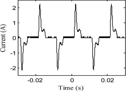
Data acquisition is achieved by using a power quality analyzer Fluke 6,105 A, from a power distorting load in Changzhou area of China. The sampling frequency is 25,000 Hz; the fundamental frequency is 50.1 Hz. The current data is still calculated with a fundamental frequency of 50 Hz, so the relative frequency deviation is 0.2%. The current waveform recorded by a power quality analyzer is shown in Fig. 4. The highest order of the harmonic measurements is 50 tones.
5.1 Verification of initial-phase sensitivity
The windows used for the experiment are still the classical cosine windows mentioned in [7], and all the time record lengths for the windowing are chosen to be the shortest analysis period.
Procedures of experimental verification are as follows: two blocks of data with different starting positions of sampling are analyzed by windowed DFT; then the signals are reconstructed in the time-domain according to the analytical results of the windowed DFT. Finally, a comparison between the two fitting curves is performed in accordance with the degree of coincidence. If the coincidence degree is good, then initial-phase sensitivity can be ignored; otherwise, initial-phase sensitivity should be considered.
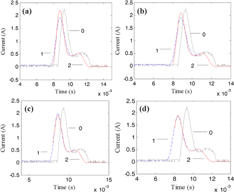
The experimental results are shown in Fig. 5. From Fig. 5(a)to Fig. 5(d), the window function used in windowed DFT is still Hanning window, Hamming window, Blackman window and 4-term Blackman-Harris window in turn. In the figure, the curve marked “0” is the original harmonic current waveform that was recorded by the analyzer, and the curves labeled “1” and “2” are the fitting curves with different starting position of sampling. Also in the following figures, the meaning of each label is identical.
The fitting curves are not coincident in Fig. 5(a) and Fig. 5(b) but coincide well in Fig. 5(c) and Fig. 5(d). Hence, initial-phase sensitivity should be considered when Hanning window and Hamming window are applied; however if Blackman window and Blackman-Harris window are adopted for windowed DFT, initial-phase sensitivity can be ignored.
Thus the experiments above have verified that initial-phase sensitivity does exist, but not all the windows used for windowing should take it into account.
5.2 Verification of the main factors influencing the initial-phase sensitivity
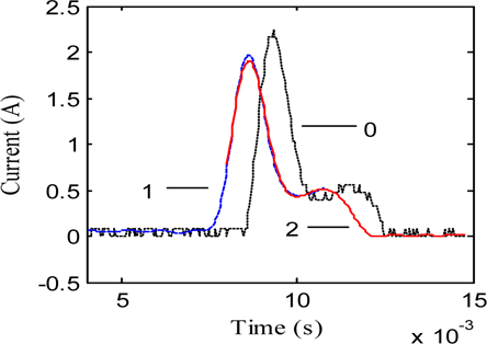
To directly confirm that the level of initial-phase sensitivity is determined by the peak side lobe level of the window, the Kaiser window(β=8) is applied. Repeating the experiment in section 5.1, the fitting curve of time is indicated in Fig. 6.
The two fitting curves coincide well in Fig. 6, indicating that initial-phase sensitivity can be neglected. Comparing Fig. 6 with Fig. 5(c), we can see the coincident degree of the two groups fitting curves are almost identical. As to Kaiser window (β=8) and Blackman window, the peak side lobe level are equal but the side lobe rolloff rate is different, therefore it is confirmed that the level of the initial-phase sensitivity is determined by the peak side lobe level.
In addition, when Blackman window and Kaiser window(β=8) are applied for windowing, the coincidence degree of the fitting curves is good. Accordingly, these experiments also prove that the peak side lobe level −58 dB can be regarded as the reference value to decide whether initial-phase sensitivity should be considered, i.e. if the peak side lobe level of window is lower than −58 dB, initial-phase sensitivity can be ignored.
5.3 Validity of increasing the time record length
Hanning-windowed DFT is selected for this experiment. The length of a data block is four periods of the fundamental component,. The experiment is repeated following the same procedures as in section 5.1.
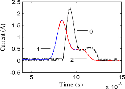
The result is illustrated in Fig. 7. Compared with Fig. 5(a), it can be seen that the method of increasing the record length is valid in reducing initial-phase sensitivity. Due to space limitations, this paper only lists the results where the analysis period is two times the length of the least period that is used in Hanningwindowed DFT. If possible, this is preferable to increasing the length of the data record.
(1) In the field test, fitting curves in the time-domain, which are reconstructed using the analytical results of windowed DFT, are not coincident with the original harmonic current waveform just because sampling is non-synchronous. So the frequency peak does not fall at frequencies that are integer multiples, leading to short-range leakage [7,15].
(2) In practical engineering, owing to the real-time requirements of harmonic measurements and restrictions on the number of discrete samples, the length of the time data is impossibly infinite. According to literature [32], when the interval is five times the length of the resolution in the frequency-domain, the spectral leakage between two harmonics can be ignored. Thus, the time length used for DFT is equal to five periods of the fundamental component, spectral leakage can then be neglected and initial-phase sensitivity is removed.
The problem of initial-phase sensitivity was discussed. DFT Windows reduce spectral leakage but cannot eliminate leakage completely, and the randomness of the initial-sampling phase makes changes to the spectral leakage, thus initial-phase sensitivity is generated. According to the results of this study, the following conclusions can be made: (1) initial-phase sensitivity has an influence on amplitude accuracy, especially for the weakfrequency harmonic components. However, not all the window functions applied in harmonic measurements need to consider this. In the case of certain synchronous deviation, initial-phase sensitivity is mainly determined by the peak side lobe level of the window: the lower the side lobe peak level the smaller the initialphase sensitivity. Initial-phase sensitivity decreases following a decrease in the peak side lobe level of the window function. There is no direct relationship between initial-phase sensitivity and the side lobe rolloff rate of the window function. (2) In practical engineering terms, the peak side level of −58 dB can be regarded as a reference value as to whether initial-phase sensitivity should be considered. If the peak side lobe level of the window function is lower than −58 dB, the error introduced by initialphase sensitivity can be ignored, otherwise initial-phase sensitivity should be considered. When a window function whose peak side lobe level is higher than −58 dB is used on the occasions that there are special requirements for weak-frequency components, the method of increasing the time record length can be chosen to remove initial-phase sensitivity. It is recommended that the record length used for windowed DFT is five periods of the fundamental component.