In recent years, nanocomposites have attracted a great deal of attention from many researchers. Several studies have shown that the incorporation of nanometric inclusions in a polymer matrix can often significantly improve its mechanical, dielectric and optical properties when compared to a pure polymer matrix [1-9], provided that the particles are reasonably well dispersed. In the electrical insulation field, polyethylene is extensively used in medium/high voltage electrical cables due to its excellent dielectric properties, very low dielectric losses and high intrinsic breakdown strength. In order to improve these properties and be able to meet new needs, such as those relating to insulation systems in DC power cables, composite materials consisting of a can be used; this results in a possible increase in breakdown strength, dielectric endurance, thermal conductivity, and allows the electrical conductivity to be tailored to avoid space charge accumulation in DC applications.
The effective permittivity of composite materials generally depends on the material microstructure, which includes the volume fraction, as well as the shapes and types of component. For some specific conditions (i.e. when the mixture has a periodic well-defined structure), the effective permittivity can be calculated from the analytical solution of the field distribution. This has resulted in various analytical models, such as the commonly used laws of mixtures. However, if the structure is disordered, as may be the case for a real compounded composite, analytical models cannot be used to accurately estimate the material’s effective permittivity. However, it should be noted that in this case, it can still be measured experimentally.
Numerical methods have been developed and calculation capabilities expanded to evaluate the effective dielectric permittivity of composite materials. Numerical simulations have in fact grown to represent another method for dealing with a large proportion of the physical problems of composite materials.
In this paper, the effective permittivity of a polyethylenebased nanocomposite is calculated by numerical simulation using the Comsol Multiphysics software, which is based on the finite element method (FEM). The influence of dispersion as well as the variation of the permittivity and radius (or the volume fraction) of inclusions on effective permittivity is studied. The electric field and polarization distribution in the nanocomposite materials are also reported in this paper. A comparison between the numerical results and those of the analytical models is presented.
The effective dielectric permittivity of a multi-phase material can be estimated either by analytical or numerical methods.
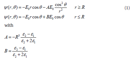
The starting point of most analytical approaches to estimating the effective properties of heterogeneous media is the solution of the single inclusion problem for which a constant field Eo along the z-direction is applied at a distance from the inclusion. This approach has been detailed in many textbooks and review papers [10-20]. In spherical coordinates, the solution of the Laplace equation for a spherical inclusion of radius R is given by:

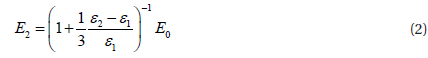
where ψ(r,θ) is the electrical potential, r is the radial coordinate, θ is the angle between the position vector and the zcoordinate, and ε1 and ε2 are the permittivities of the inclusion and the matrix, respectively. It should be noted that the same equations hold in steady-state AC conditions in which the potential would be a phasor and the permittivity can take complex values, including a possible conductivity term. The electrical field along the z-direction inside the inclusion according to (1) is given by:

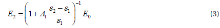
A similar calculation can be made for the more general case of an ellipsoidal inclusion leading to:

where A1 is the depolarization factor along the ellipsoid principal axis parallel to the electrical field [11]. For spherical particles, A1 = A2 = A3 = 1/3 and (3) is identical to (2). By definition, the effective dielectric constant of a two-component heterogeneous linear material can be defined by [21]:

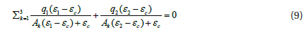
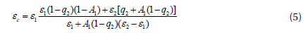
where εc is the effective permittivity, q1 and q2 are the volume fraction of the matrix and the inclusion, and the brackets denote averages over phase 1, phase 2 and over the material’s volume. An analytical calculation of the electrical field in a composite material can only be done if the minority phase is present in a small concentration and has regular shape inclusions. A number of results can be found in which an exact solution for several matrix systems with periodic arrangements of regular inclusions is obtained [22,23]. In the case of a dilute suspension of ellipsoidal shape inclusions with a permittivity ε2 in a continuum matrix of permittivity ε1, it is possible to use the solution of the singleinclusion problem (equation (3)), assuming that the field Eo is equivalent to the average field in the matrix (phase 1). This leads to [11]:
A similar procedure leads, for randomly oriented inclusions, to:
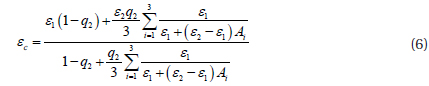
where Ai is the depolarization factor for the ith axis of the ellipsoid. For spherical particles, A1 = A2 = A3 = 1/3. In the case of spheroids for which two axes are equal (a = b ≠ c), the analytical expressions for Ai for oblate spheroids (disk-like spheroids with a = b > c) and prolate spheroids (needle-like spheroids with a = b < c) can be found in literature [10].
Another approach, the effective medium approximation, also relies on the solution of the single-inclusion boundary value problem. The generalization of the Maxwell approximation for ellipsoidal inclusion leads to:
for a two-phase composite consisting of a perfectly oriented ellipsoidal inclusion (phase 2) inside a matrix (phase 1). It can be shown that this equation is equivalent to equation (5), and the randomly oriented case would be equivalent to (6). This is also the exact solution of the coated-spheres model [24].
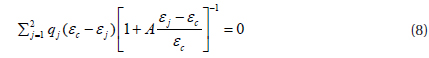
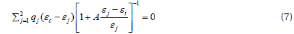
A different approach in the effective medium approximation family is the self-consistent approximation, which was originally developed by Bruggeman [25]. It leads to a slight modification of (7):

which in turn leads to a quadratic equation for the effective permittivity. For the case of the randomly oriented ellipsoidal, equation (8) can be written [26] as:

Finally, using a symmetric integration technique [27], it can be shown that the Looyenga equation for randomly oriented ellipsoids, independent of their shape, is given by:

As mentioned previously, all the above equations also hold in steady-state AC conditions. In this case, the electric fields can be replaced by their respective phasors and the permittivity can be replaced by their complex representation. Accordingly, equations (5) to (10) can also be used to predict a composite dielectric response, i.e., the variation of the effective complex permittivity as a function of frequency, by replacing ε1 and ε2 by their frequencydependent complex representations.
The effective permittivity of the dielectric mixture can be calculated once the electric field vector is known inside the material. In a purely electrostatic case, it can be calculated by solving the Poisson's equation given by:

where εr, ε0 and Ψ are the relative permittivity, the vacuum permittivity and the electrical potential, respectively. ρ is the charge density. For the neutral condition (ρ = 0), and if we take into account a possible conductivity σ and dielectric losses, then (11) can be written in the steady state more generally as [28-30]:

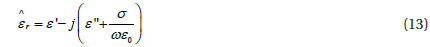
where the complex permittivity is given by:

Once the material microstructure and the properties of each phase are known, (11) or (12) can be numerically solved by the finite elements method (FEM) using a commercially available package like COMSOL Multiphysics. After the field distribution is numerically evaluated, the effective permittivity of the dielectric mixture can be calculated in several ways [30-38]. In this paper, the effective dielectric permittivity of the composites was calculated by using the averages of the electric field and dielectric displacement values. Therefore, the effective dielectric permittivity can be expressed as follows:
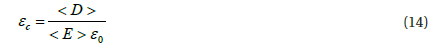
where <
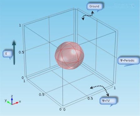
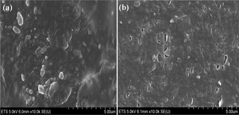
The morphology of polyethylene/clay nanocomposite in the nanometric scale observed by scanning electronic microscopy (SEM) is shown in Fig. 1. As can be seen, two components are presented in the nanocomposite. This two-phase nanocomposite consists of 5 wt% of nanoclay particles dispersed in a polyethylene matrix. A comparison between the morphology of polyethylene with 5 wt% nanoclay, PE/O-MMT (Fig. 1(a)), and polyethylene with 5 wt% nanoclay and 10 wt% of compatibilizer, PE/O-MMT/PE-MA (Fig. 1(b)), shows that the density and size of aggregates were decreased in the compatibilized nanocomposite. This improvement in the nanoclay dispersion is due to the presence of the polar compatibilizer, PE-MA [8]. In this paper, the dielectric permittivity of the polyethylene matrix and that of the nanoclay reinforcing fillers are taken to be as follows: ε1=2.3 and ε2=4.4, for the matrix and the filler, respectively. A singleinclusion 3-D model cell was used as a first approach, as shown in Fig. 2. The inclusion was assumed to have a spherical form to simulate the shape of a nanoclay particle, and the radius of this was later calculated in order to meet the requirement of a 5% volume fraction of the particles. The bottom face of the cube was set to a constant potential (Ψ = 1 V), and the opposite face was set to ground (Ψ = 0). The other faces of the cube were set to periodic conditions.
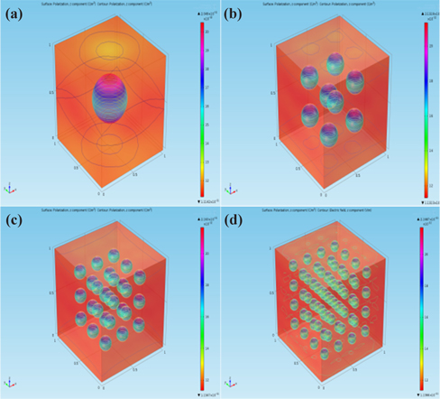
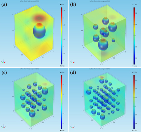
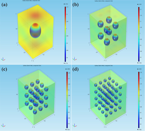
In order to study the effect of the dispersion of nanoclay particles on dielectric properties, such as electric field distributions and effective permittivity, four geometries (with the same volume fraction q=0.05) were drawn with 1, 8, 27 and 64 spheres corresponding to particle normalized radii of 0.229, 0.114, 0.076 and 0.057 (Figures 3(a)-3(d)).
The surface plots of the electric field distribution in the 3-D model were obtained by FEM simulations, and are shown in Fig. 3.
As can be predicted by the single-inclusion solution, a field enhancement is present at the interface between the particle and the matrix on the bottom and top sides in the z-direction, the field is almost constant and smaller within the inclusion. The maximum value of the electric field Emax increases as the degree of dispersion of the nanoclay particles increases, and the highest value is obtained when the number of spheres is 27.
The polarization vector (in C/m2) distributions for all 4 geometries are shown in Figure 4, along with an enhancement at the matrix-particle interfaces in the z-direction. The highest value of polarization was found at the surface of the particles in the cell with 64 spheres. It is evident from the images that the polarization increases as the degree of dispersion of the nanoclay particles increases.
In the above section, the uniform reinforcing particles are considered to be orderly dispersed in a polyethylene matrix. In real materials, nanoclay particles or any reinforcing filler are distributed more or less randomly in the polymer matrix with agglomerate size distributions. Figures 5(a)-Figures 5(d) show four geometries and electric field distribution plots for different numbers of randomized nanoclay particles. The volume fraction of nanoclay particles was set at 5% and dispersed in a unit cell.
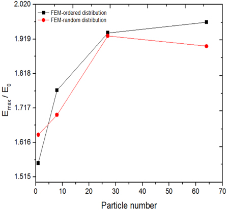
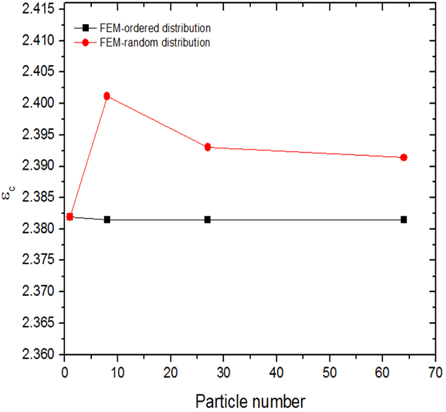
The corresponding effective permittivity and normalized maximum electric field Emax/E0 (where E0=1 kV/mm) of the nanocomposite materials are plotted in Figs. 6 and Figs. 7, respectively. As can be seen from Fig. 6, the effective permittivity for ordered distributions does not vary significantly with the number of particles. This is due to the fact that the volume fraction of nanoclay particles was constant and set at 5%. On the other hand, the effective permittivity of the random distribution was found to be higher than that of ordered distributions. This change is due to a decrease of the distance between inclusions in the random distribution.
Figure 7 shows the normalized maximum value of the electric field in the z-direction as a function of the particle dispersion. At a low particle number, it can be seen that the normalized maximum electric field is almost identical for the ordered distribution as for the random cases, and we can also see it increases as the quality of dispersion is improved. For particle numbers higher than 27, the normalized maximum value of the electric field in the random distribution decreases slightly as the quality of dispersion increases, while in the ordered distribution, the electric field is found to increase considerably with an increase in the number of particles.
3.4 Effect of the permittivity of the inclusion on effective permittivity
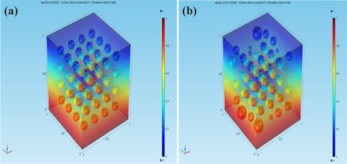
In this section, the two geometries of 64 spheres of the ordered and random distributions presenting the distribution of the electrical potential simulated by FEM are shown in Figs. 8(a) and 8(b) to show the effect of a variation of the dielectric permittivity of inclusions on the effective permittivity of the ordered and random nanocomposites. The resulting effective permittivities obtained from FEM are compared with those calculated from equation (7), the Maxwell-Garnett model, equation (9), the Brug In this section, the two geometries of 64 spheres of the ordered and random distributions presenting the distribution of the electrical potential simulated by FEM are shown in Figs. 8(a) and Figs. 8(b) to show the effect of a variation of the dielectric permittivity of inclusions on the effective permittivity of the ordered and random nanocomposites. The resulting effective permittivities obtained from FEM are compared with those calculated from equation (7), the Maxwell-Garnett model, equation (9), the Bruggeman model, and equation (10), the Looyenga model.
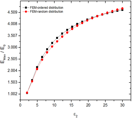
Figure 10 shows the effect of varying the permittivity of the inclusion ε2 on the normalized maximum value of the electrical field in the z-direction. As expected, for ordered and random distributions, the maximum value of the electrical field increases as the value ε2 increases.
3.5 Effect of the radius (and volume fraction) of the inclusion on effective permittivity
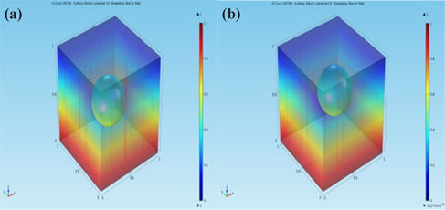
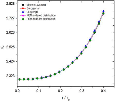
The distributions of the electric potential simulated by FEM for the two geometries for the single-inclusion case, of the ordered and random distributions, are shown in Fig. 11. In the simulation, the permittivity of the polymer matrix ε1 is still assumed to be 2.3, and the permittivity of the inclusion ε2 is set at 4.4. To study the effect of nanoclay loading on the effective permittivity εc, the normalized radius of the inclusion r/r0 (where r0=1 μm) was varied from 0.010 to 0.400, corresponding to a volume fraction of nanoparticles ranging from 0.0004% to 26.81%.
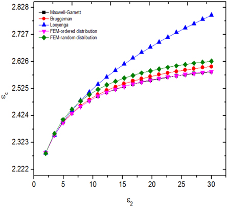
The effective permittivity of the nanocomposites as a function of the radius of nanoclay particles is plotted in Fig. 12. It can be observed that the effective permittivity increases with the nanoclay particle radius, and it is evident from this figure that the effective permittivity of the ordered and random distributions obtained from FEM is quite similar to that calculated with the Maxwell-Garnett model, and is also very close to those of the Bruggeman and Looyenga models. These results confirm the validity of our simulation method.
A 3-D simulation model using the finite elements method was developed in order to study the effective permittivity and electric field distribution of polyethylene/clay nanocomposite materials for electrical applications. An enhancement of the electric field and polarization was observed as the degree of dispersion of the nanoclay particles increased; however, the effective permittivity of the nanocomposites was not affected by improving the quality of dispersion of nanoclay particles in the host matrix. The numerical results indicate that the Maxwell-Garnett model is appropriate for evaluating the effective permittivity of ordered distributions, while the Bruggeman Symmetry model remains the most suitable for calculating the effective permittivity for random distributions. It was observed that in both distributions the maximum value of the electrical field and the effective permittivity εc increase as the value ε2 increases. Finally, this numerical model can be extended to design nanocomposite materials with optimum dielectric properties for electrotechnical or electronic applications.