The solar cells are connected in series or parallel as a module to generate stable and durable power from the external environment. A power drop, compared with the sum of each solar cell output power, occurs because of increased resistances. A power mismatch [1] occurs under a shaded condition [2].
The output power of PV module was predicted by a theoretical approach that considers the resistance factor. This approach uses the parameters, Voc, Isc, Vmp, and Imp, and the temperature coefficient to obtain series resistance, shunt resistance and reverse saturation current, essential for predicting output power. Also, it predicts the variation of output power due to irradiance. Maximum errors of 1.27% in current and 0.74% in voltage are shown between the theoretical predicted result and the experimental result obtained by using the MATLAB program. Moreover, we investigate the connections of mismatched cells and obtain an I-V equation. Maximum errors of 3.11% in current and 0.76% in voltage occur at the mismatched connections. A power drop of 15.13% is shown for the series mismatched connection, which is greater than that for the series normal connection, and a drop of 9.36% is shown for the parallel mismatched connection, which is greater than that for the parallel normal connection. Thus, it is useful to predict the output power in a mismatched connection when PV modules are manufactured.
2. PREDICTION OF PV MODULE OUTPUT CHARACTERISTICS
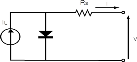
A PV module operates similar to a solar cell, so the I-V equation was derived from the I-V equation for a solar cell. The current equation, as well as the series resistance and shunt resistance, of a PV module is introduced in this chapter [3,4].
A PV module has a number of solar cells connected in series or connected in parallel. A module parameter was subject to the parameters of solar cells in the module.
where IM is the PV module current and NP, IscM, VM, NS, VocM, RsM, and RshM are the number of parallel strings or cells, short circuit current, voltage of the module, number of series-connected cells, open circuit voltage, series resistance, and shunt resistance, respectively, where the subscript M denotes “module”. The equation of the PV module current is developed by using these values.
From equation (2.8), the undefined IsM, RsM and RshM were found by the following steps. First, if the shunt resistance is infinite, the equivalent circuit becomes a simple circuit that was represented by using Eq. (2.9), and it was further transformed into Eq. (2.10).
The equation of Is for a module is obtained by placing a zero into the equation instead of I because VM=VocM when IM=0 in Eq. (2.10).
Next, the fill factor is used to obtain the PV module series resistance (RsM), and we assume that the unit fill factors of a PV module (FFoM) and solar cell (FFo) are equal [5,6].
Eq. (2.13) shows a rearranged equation of Eq. (2.12) by using Green’s theorem, and it is meaningful when the value is greater than 10.
where γsM is the normalized resistance that leads to the decrease in the fill factor.
where Vmp' is the ideal maximum power voltage and Imp' is the ideal maximum power current. Eq. (2.16) was expressed by Eq. (2.19) and applied to the fill factor.
Eq. (2.15) is expanded to Eq. (2.20). Eq. (2.21) shows the maximum power of the PV module and from this equation, RsM is obtained.
Finally, RshM was obtained by using the values of PmaxM. To obtain RshM, Eq.(2.8) was calculated with changing value of RshM until calculated P_maxM is similar to measured PmaxM within 0.4% error. In the following chapter, this simulation is explained in detail. To prove the theory so far, MATLAB is utilized by using four factors from a real PV module and the Lambert W function [7].
The PV module current is then calculated by changing the PV module voltage from 0 to Voc. The diode ideality factor (n) is changed according to the solar cell characteristics [7]. In this simulation, the ideality factor is 1.4 when VocM divided by the number of solar cells in a module is greater than 0.6[V]. Otherwise, when the voltage is less than 0.6[V], the ideality factor is 1.8.
3. ANALYSIS OF PV MODULE INTERCONNECTION CHARACTERISTICS
3.1 Mismatched connection in parallel
To simplify the equation of the mismatched connection in parallel, two cells are initially used in parallel. The normalized I-V equation of the cells is shown below and the subscript represents the number of cells.
Eq. (3.2) is induced when V is a variable, so we use V1=V2.
Eq. (3.2) can be expanded to Eq. (3.3) when NP solar cells are connected in parallel.
3.2 Mismatched connection in series
The total current is easy to calculate when a deficient cell is connected in parallel, but difficult to count when a deficient cell is connected in series because the equation expands in terms of voltage. For this reason, Eq. (2.1) should be rearranged in terms of current as below.
VT, defined as V1+V2, is the total voltage drop in a series connection, obtained from Eq. (3.4) as follows.
If the electrical characteristics used in the connection are identical, Eq. (3.5) can be rearranged as follows.
Eq. (3.6) is expanded to Eq. (3.7) when Ns solar cells are conocnected in series under the assumption of same electrical characteristics.
Eq. (3.7) is expressed in terms of current as
The comparison of Eq. (3.8) and Eq. (2.8) shows that the shunt resistance (RshM) of the PV module is equal to that of the solar cell (Rsh). Ns cells and one deficient cell are connected in series to extend the model to a real application. The value of Ib can be changed to IT when I is a variable in Eq. (3.9), so the I-V characteristics in this connection can be predicted. The new total voltage equation is
where Iscb, Ib, Rsb, Rshb, Isb and Rb represent the short circuit current, total current, series resistance, shunt resistance, reverse saturation current and total resistance of a deficient cell, respectively.
3.3 Simulation of I-V characteristics of the cells
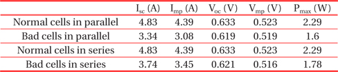
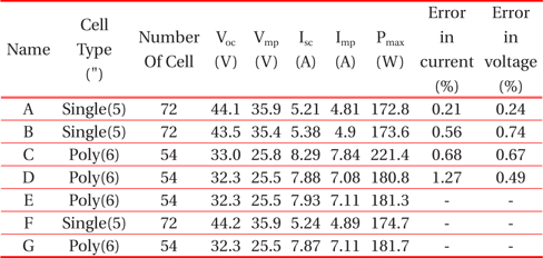
Simulation was carried out based on the theory introduced to confirm the effect of the electrical mismatch of solar cells in a PV module. The sample for the experiment consisted of three solar cells and their characteristics are provided in Table. 3.1. The parameters from Table 3.1 were obtained by using a solar cell tester, CT801. Also, the values Rs, Rsh and Is in Table 3.2 were extracted from the results of the cells that were simulated for the introduced model by using the parameters from Table 3.1. The value of Pmax is used to distinguish normal and bad samples in Table 3.1.
[Table 3.1.] Parameters of solar cell for simulation.

Parameters of solar cell for simulation.
[Table 3.2.] Physical parameters of solar cell obtained from the simulation.
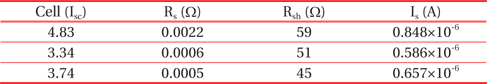
Physical parameters of solar cell obtained from the simulation.
3.3.1 Mismatched connection in parallel
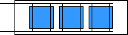
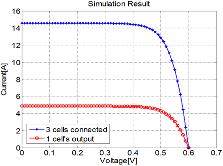
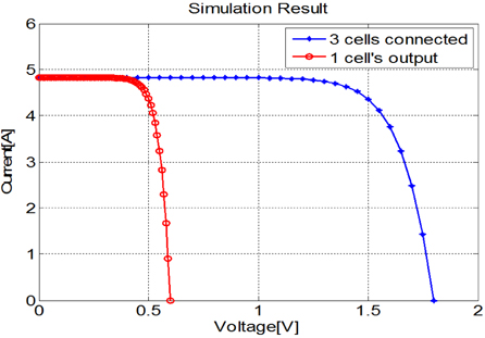
Figure 3.1 shows the parallel connection of normal solar cells. Because the cells have the same characteristics, the equation of IT=I1+I2 was used. Figure 3.2 shows the I-V characteristic of a normal cell and a PV module of three normal cells. As predicted, the output voltages are the same and the current value of the PV module is three times the current of the solar cell. The parameters from Table 3.2 are used for the simulation.
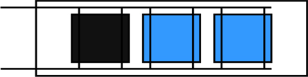
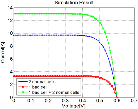
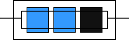
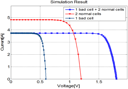
Figure 3.3 shows a parallel connection of 2 normal cells and 1 deficient cell, which has the same voltage characteristic as a normal cell but a poor current characteristic.
Figure 3.4 shows the simulation result of the connection in Fig. 3.3. The total current value is lower than that shown in Fig. 3.2 because of the deficient cell.
3.3.2 Mismatched connection in series
Eq. (3.9) is rearranged in the following steps from Eq. (3.10) to (3.12) to simulate a series connection. The voltage value was calculated by using the current change starting from 0. In the case of common I-V curve of a module, the current value is almost constant as Isc although the voltage value is changing at the low voltage region. The general PV module equation expressed by the current equation does not have a problem because the voltage value is changed, and the current value is then obtained from the voltage change. However, the result from calculated voltage equation (3.11), a current variable, is an imaginary quantity after starting point which the current is saturated as Isc. Therefore, the voltage value is calculated by Eq. 3.11
where Ns is the number of normal cells and M is the correction factor that make the two equations give the same value at the interconnection point. M is approximately 0.05~1.5, and this work uses 0.1. Iscsum is the total number of normal cells and deficient cells. The normalized voltage equation that ignores the resistance factor is shown below and the subscript
The equation I=Isc is valid whenV1+V2=0 in Eq. (3.14) , so Iscsum is defined as a current when VT is zero.
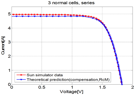
The valid value is that with the minus sign before the root in Eq. (3.15); this result means that the total current value follows the lowest value, the current of the deficient cell. Fig. 3.5 shows the I-V characteristics of a normal cell and a PV module with three normal cells in series. The output current values are the same, but the output voltage value of the PV module is three times greater than that of the cell.
Figure 3.6 shows a series connection of 2 normal cells and 1 deficient cell that has the same voltage characteristics as the normal cells but poor current characteristics.
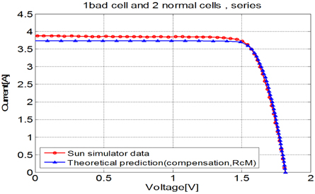
Figure 3.7 shows the simulation result of the connection in Fig. 3.6. The total current value is less than that of a PV module with three normal cells due to the one deficient cell.
4.1 PV module output characteristic prediction
Seven types of PV modules are tested to prove the proposed equation and to compare their I-V characteristics with the theoretical predictions. Table 4.1 shows the parameters of the PV modules, the numbers of cells and the error between theoretical and experimental data for 1,000 W/m2 irradiance.
[Table 4.1.] parameter of PV module for comparison.

parameter of PV module for comparison.
The measured and simulated I-V characteristics of four samples ‘A’, ‘B’, ‘C’ and ‘D’ are compared for 1,000[W/m2] irradiance. Current deviation is calculated at the voltage lower than Pmax, and voltage deviation is also counted at the voltage higher than Pmax.
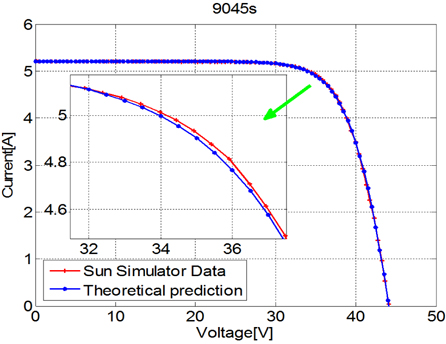
Figure 4.1 shows the result of the ‘A’ module, which has the maximum errors of 0.21% in current and 0.24% in voltage.
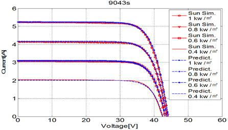
The result shows that the sun simulator data and theoretical prediction data at 1,000 W/m2 irradiance are matched well in Fig. 4.1. The maximum errors of 1.27% in current and 0.74% in voltage are shown. To prove the proposed equation by irradiance variation, simulated and measured results are compared at irradiances of 1,000 W/m2, 800 W/m2, 600 W/m2 and 400 W/m2 with ‘E’, ‘F’ and ‘G’ samples, and the temperature of the PV module is assumed as 25℃. Figure 4.2 describes the result of the ‘F’ module that has maximum errors of 1.32% in current and 0.48% in voltage.
The simulation by irradiance needs to consider series resistance, so it is assumed that series resistance decreases as the irradiance reduces. This assumption is applied to Eq. (4.1). This new equation is used for the experiments according to irradiance.
where rIrr is the ratio of real irradiance to standard irradiance, RsM' is the new resistance according to irradiance, α is the correction factor that considers ribbon resistance, which is usually 0.8~1.2 but in this work, is set to 1.0. Moreover, the short circuit current is compensated in Eq. (4.2) because the short circuit current decreases non-linearly with irradiance reduction. Eq. (4.2) provides more accurate results and is good agreement with measured output of a module, shown former example.
where IscM' is the new short circuit current that considers irradiance, β is that correction factor that considers the absorbance coefficient and generation rate of irradiance, which is normally 0.02~0.03. In this paper, the correction factor is 0.025.
The irradiance variation affects the value, VocM, which is related to the short circuit current and reverse saturation current. The reverse saturation current, which is defined by Eq. (2.11), has an open circuit voltage value at the irradiance of 1 kW/m2. The open circuit voltage should change with irradiance, so the new equation is therefore developed below.
where VocM is the open circuit voltage at the irradiance of 1 kW/ m2, VocMIs is the imaginary open circuit voltage according to irradiance in the PV module, which is proposed to obtain the reverse saturation current, and δ is a correction factor that considers the variation of voltage according to irradiance, which is normally 0.02~0.05 but is 0.033 in this work.
4.2 Comparison results between theoretical and measured data
The PV modules manufactured for the experiment were tested, and the measured results were compared with the simulated data from the previous chapter. One of the PV modules had three normal cells and the other one had two normal cells and one deficient cell. The modules were not laminated; only the solar cells were connected onto the glass. The parameters from the solar cells were obtained in the simulation, but when the PV module was made, an electrode ribbon and interconnection ribbon were used. Therefore, the resistance from the modulation process should be considered when the parameters are obtained only from the solar cells. The following equation represents the open circuit voltage of a PV module that has a smaller value than the total sum of the open circuit voltages of all cells due to contact resistance.
Where RcM is the increased value of the contact resistance; 0.005 Ω was used for series and parallel connections in this work. However, the contact resistance of the parallel connection is greater than that of the series connection because the ribbon is used more frequently in parallel connection. Eq. (4.5) shows this consideration.
where RsM' is the resistance that considers the increased value of the contact resistance and RcLM is the increased value of contact resistance according to the number of parallel connections and the method of soldering. The value of RcLM is normally 0.01[Ω] ~ 0.1[Ω] ; 0.02[Ω] was in this work. When the solar cells were connected in parallel, the series resistance of 0.02[Ω] was used for simulation. Similar to the method shown in the former chapter, the current deviation is compared at the voltage lower than Pmax, and the voltage deviation is compared at voltage higher than Pmax.
Figure 4.3 shows the I-V characteristics of the theoretical prediction and the sun simulator data of a PV module with three solar cells in series. The result shows the maximum errors of 2.56% in current and 0.29% in voltage. Also, the simulated value of PmaxM is 6.61W and the theoretical value is 6.52[W], showing an error of 1.36%. Figure 4.4 shows the I-V characteristics of the theoretical prediction and sun simulator data of a PV module with 1 deficient cell and 2 normal cells in series. The result shows the maximum errors of 3.11% in current and the 0.58% in voltage. Also, the simulated value of PmaxM is 5.61[W] and the theoretical value is 5.55[W], showing an error of 1.07%.
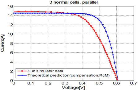
Figure 4.5 shows the I-V characteristics of the theoretical prediction and sun simulator data of a PV module with 3 solar cells in parallel. The result shows maximum errors of 2.56% in current and 15.10% in voltage. A significant error in voltage is shown because only the open circuit voltage with increase in contact resistance is considered. Therefore, the series resistance shows a significant difference, resulting in the large error in voltage.
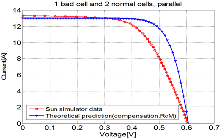
Figure 4.6 shows the I-V characteristics of the theoretical prediction and sun simulator data of the PV module with 1 deficient cell and 2 normal cells in parallel. The result shows maximum errors of 2.56% in current and 14.04% in voltage. This result also shows a large error in voltage for the same reason as that in Fig. 4.5. These errors result from additional resistances in parallel connection due to the longer electrode and interconnection ribbons. Simulations were then performed by considering those additional resistances.
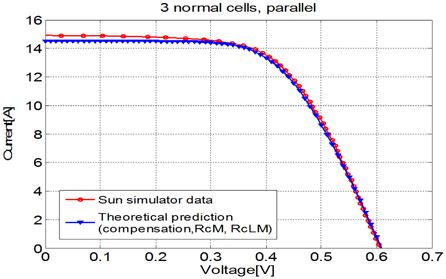
The I-V characteristics of Fig. 4.7, which include the increase in contact resistances of electrode ribbon and interconnection ribbon, are different from those of Fig. 4.5. While these results are more accurate accounting for the increase in contact resistance, they still show slight errors. The result shows maximum errors of 2.56% in current and 0.76% in voltage. Also, the simulated value of PmaxM is 5.45[W] and the theoretical value is 5.36[W], showing an error of 1.65%.
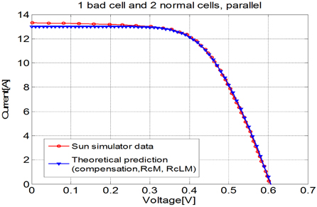
The I-V characteristics of Fig. 4.8, which also considers the increase in contact resistances of electrode ribbon and interconnection ribbon, are different from those of Fig. 4.6. The result shows maximum errors of 2.26% in current and 0.55% in voltage. Also, the simulated value of PmaxM is 4.94[W], and the theoretical value is 4.91[W], showing an error of 0.61%.
The difference in the output power between the PV module with 3 normal solar cells and the mismatched PV module is 9.36% for the sun simulator result and is 8.41% for the theoretical result. These values are slightly smaller than those of the PV modules with the series connection. The results are summarized in Table 4.2.
[Table 4.2.] Errors of different interconnections.
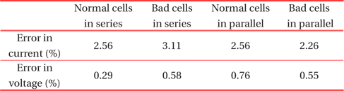
Errors of different interconnections.
The parameters Voc, Isc, Vmp, and Imp and the temperature coefficient were used to obtain the series resistance, shunt resistance and reverse saturation current of a PV module, which are essential for predicting the output power of a PV module. The proposed equation worked well with the results according to the amount of irradiance. When the irradiance was 1,000 W/m2, maximum errors of 1.27% in current and 0.74% in voltage were obtained between the theoretical predicted output and experimental output. Moreover, the maximum errors changed to 1.88% in current and 1.71% in voltage when the irradiance was changed. The change of series resistance according to irradiance was considered and short circuit current according to irradiance was approached practically. Also, a new equation for the open circuit voltage to analyze the reverse saturation current was proposed.
The theory proposed, which can predict output characteristics by the interconnection method, was verified by comparing the measurements of the real PV module with the 3 solar cells in series and in parallel. Increasing contact resistance, which induced the decrease of the open circuit voltage, was considered when the solar cells were connected. Furthermore, the additional contact resistance in parallel connection due to a longer electrode ribbon and interconnection ribbon was considered. Therefore, the results from the new equation and the data from a real PV module were similar.
The standard of current differed between a cell tester that simulates a solar cell and a sun simulator that simulates a PV module. Current value comparisons are somewhat inaccurate, but maximum errors of 3.11% in current and 0.58% in voltage occurred. The maximum error of 2.55% in current was shown for a parallel connection when only the contact resistance was considered as a series connection, but a significant error of 15.10% in voltage occurred. Therefore, the additional series resistance for a parallel connection was included to obtain better results: maximum errors of 2.56% in current and 0.76% in voltage. An output power drop occurred when a deficient cell was connected in this work. The drop rate was 14.88% for a series connection and 8.40% for a parallel connection.
This work will be helpful in analyzing the characteristics of a degraded PV module and in predicting the output power, which is critical at PV power stations, when cells gradually degrade in PV modules.