Data clustering is an important task in many areas, as such many clustering algorithms have been developed. However, many of these are neither effective nor efficient for data points in high dimensional spaces. There are several main reasons for this. Firstly, the inherent sparsity of high dimensional data hinders conventional clustering algorithms. Secondly, the distance between any two points becomes almost the same in high dimensional space [1], therefore it is difficult to differentiate similar data points from dissimilar ones. Thirdly, clusters are often embedded in subspaces of high dimensional space, and different clusters may exist in different subspaces [2].

Image clustering is a typical application of high dimensional clustering algorithms, this is because for image features nearly all the dimensions are high. So, the problem of high dimensional clustering is very apparent in image clustering applications. What’s more, the scale of an image dataset is generally large, and this scale may also change in some online applications. The performance of conventional clustering algorithms deteriorates significantly when used on this kind of dataset. For example, k-means is the mainstream cluster method in the image visual bag of words model for visual dictionary construction. However, when the number of images is large, the time taken to cluster is very long and may even be unacceptable for practical purposes. On top of this, when the image data is ever increasing, re-clustering is needed for k-means as it is not a dynamic cluster method. These limitations of k-means seriously damage its feasibility for use with large incremental image datasets. Some improvements to k-means, such as hierarchal k-means [3] and approximate k-means [4], have been presented, however, these have been shown not to support dynamic clustering [5]. Currently, widely used clustering methods such as spectrum clustering [6] and Affinity Propagation [7] methods incur high memory and computation costs due to the matrix factorization that they require. Therefore, a more efficient, new cluster method is needed.

Random projection is used in many areas including fast approximate nearest-neighbor applications [8,9], clustering [10], signal processing [11], anomaly detection [12] and dimension reduction [13]. This is largely due to the fact that distances are preserved under such transformations in certain circumstances [14]. Moreover, random projections have also been applied to classifications for a variety of purposes [15, 16].

E²LSH(Exact Euclidean Locality Sensitive Hashing) is a special case of random projection, and it was first introduced as approximate near neighbor algorithm [17]. E²LSH has attracted much attention recently, and has mainly been used in retrieval [18, 19]. In fact, the data points projected into the same buckets were found to be much more similar than those projected into different buckets. So, if we take a dataset and divide into groups according to its bucket indices, the task of data clustering has already be achieved to a certain approximation. What’s more, E²LSH is a data independent method, so it can create a dynamic index for an incremental dataset. In this way, E²LSH can be used as a dynamic clustering method. In fact, the introducer of LSH has pointed out that LSH can serve as a fast clustering algorithm, but he did this without going on to validate the claim. In fact, E²LSH has even been applied to noun clustering by Ravichandran D [20]. However, clustering image data is more difficult than text word data because of its added complexity.

Therefore, we proposed an enhanced Locality Sensitive Clustering (LSC) method for use in high dimensional space based on E²LSH. This method takes advantage of Locality Sensitive Hashing (LSH) and can cluster high dimension data at a high speed.

The main property of random projection is dimension reduction. Compared with the classical dimension reduction algorithm PCA (Principal Component Analysis), random projection offers many benefits [21]. For example, generally PCA can’t be used to reduce the dimension of a mixture of n Gaussians to below (Ωn), whereas random projection can reduce the dimension to just Ω(log n). Random Projection has another tremendous benefit, even if the original Gaussians are highly skewed, their projected counterparts will be more spherical. This is a great advantage as it is much easier to design algorithms for spherical clusters than ellipsoidal ones.

As for data clustering, the Johnson-Lindenstrauss Lemma shows that the distances to data points are preserved after projection. This makes it capable for use in approximate nearest neighbor search when performing information retrieval.

The Johnson-Lindenstrauss Lemma is famous for its distance preservation property. It can be described like this: Given 0<ε<1 and any set S in ℝⁿ, for a positive integer , there exists a map f : ℝⁿ → ℝ^d, such that for all u,v ∈ S,

This lemma says that all pairwise distances are preserved, with high probability, up to 1±γ after mapping.

Let N(0,1) denote the standard normal distribution with mean 0 and variance 1, and U(-1,1) denote the distribution that has the probability 1/2 on -1 and probability 1/2 on 1.

Let u,v∈Rⁿ, and where A is the random matrix, whose entries are chosen independently from either or . Then

Imagine a set S of data in some high-dimensional space Rⁿ, and suppose that we randomly project the data down to R^d. By the Johnson-Lindenstrauss Lemma, d = O(γ^-2 log|S|) is sufficient so that, with high probability, all angles between points change by at most ±γ/2 [22]. In particular, consider projecting all points in S and the target vector ω, if initially data was separable by margin γ, then after projection, since angles with ω have changed by at most γ/2, the data will still be separable.

E²LSH is a special case of LSH (Locality Sensitive Hashing), and it is a random projection based method. This can be illustrated by the definition of the hashing function. The k hashing functions are generated by random methods, and their innerproduct performs the data projection. This, however, is different from general random projection, because each data point is projected by k hashing functions, and as such results in k bucket indices that represent an original point. The k hashing functions also indicate a difference from general random projection in two ways. The first is the projection itself, the projection was not performed on the whole axis in one direction, but on parts of the axis. The second is that general projection is done by a matrix operation (a data point multiplies a n×d random projection matrix A), but in E²LSH, a data point multiplies a single hashing vector, as such the matrix operation is omitted in E²LSH. This is of vital importance for large-scale data processing, because the multiple matrix operations needed by traditional algorithms are impractical due to high computation and memory costs.

E²LSH can also be used for data clustering. Based on the separability description above, we can say a dataset’s distance, margin and angle could be preserved after projection. These properties make E²LSH feasible for data clustering. In fact, the bucket indices found after projection can be used to group data points. This comes from the fact that similar data are arranged into a single bucket or the adjacent several buckets. So if we group these into a cluster, and further group all similar groups into corresponding clusters, the goal of data clustering can be achieved. This is the main idea behind Locality Sensitive Clustering.

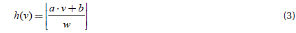
E²LSH is based on the p - stable distribution function, its single hashing function is defined as:

where a is a n-dimension vector generated by the p - stable distribution function, and the inner-product (a·v) works as a single channel random projection, b is the offset added to the random projection, and the module operation ensure the projected value (bucket index) is in a specific range.

The projection function is similar to LSH and projects points in ℝⁿ to ℝ^k:

The enhanced Locality Sensitive Clustering (LSC) includes several main steps. Firstly, optimal parameters k and L are computed. Secondly, the hashing function for point v is constructed. Thirdly, all points are projected to bucket index (h₁,···h_k), and the bucket indices of all points are clustered to get the cluster labels. The procedure for enhanced Locality Sensitive Clustering (LSC) is shown below:

Step 1, the optimal parameters k and L are calculated for a dataset S. Step 2, k dimension vector A is generated from the Gaussian distribution, b and w are also generated according the definition of the LSH function. Step 3, all the points vi∈S are projected to a k dimension bucket index Bi, and these bucket indices constitute a matrix B. Step 4, randomly selected one column Bj from matrix B, and cluster bucket indices Bj to get n clusters where j∈[l,m], m=|S| and n is the number of clusters.

where l_k denotes the cluster labels, l_k = k, k∈[1,n], n<m. Step 5, assign points in B_j to class k

where B_j^-1 denotes the points whose bucket index is B_j.

To verify the effect of the new clustering method on real data, we constructed an image set from the TRECVID image dataset, the set contains four categories and 75 images total. The 4 categories are ‘compere’, ‘singer’, ‘rice’ and ‘sports’.

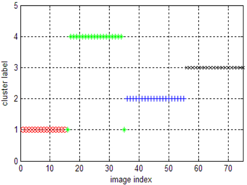
To compare the performance of our new algorithm, we first ran k-means on this image set. The results of k-means on the image dataset are showed in Fig. 1.

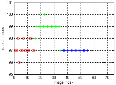
The result of LSC on the image dataset is shown in Fig. 2. Most of the cluster labels in cluster 2 and 4 are correct, the clustering labels of cluster 3 are correct while several cluster labels of cluster 1 are wrong. We can see that the accuracy of clustering labels are less than in the synthetic data, this is because the distinctness of inter-clusters are less than in the synthetic data. However, results on real data are more meaningful.

As LSC is a randomized algorithm, it is understandable that its clustering results are less accurate than k-means. On the other hand, the advantage of LSC lies in its low computation cost, fast running speed and the dynamic clustering which comes from E²LSH.

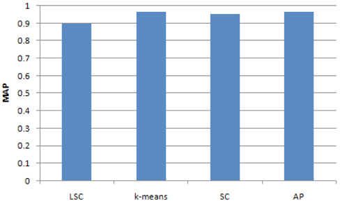
To compare the accuracy of the two methods, we computed a MAP of the clustering results for the 4 classes using LSC, k-means, Affinity Propagation (AP) cluster and Spectrum Cluster (SC) methods. The results are showed in Fig. 3. It can be seen that the accuracy of LSC is about 0.9, which is less than k-means, AP and SC.

To compare clustering times, we ran the four cluster methods (LSC, k-means, AP cluster and SC) on the image dataset. The results are showed in table 1. It can be seen that LSC consumes the least time while AP and SC cost significantly more time than LSC and k-means.

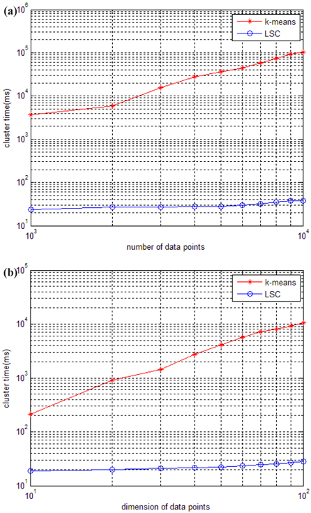
To conveniently see the running time of our new clustering method, we construct a synthetic dataset 1 and synthetic dataset 2. Synthetic dataset 1 is an incremental dataset in scale, which contains 5 clusters of 100 dimension pieces of data, the number of data points increases from 1,000 to 10,000. Synthetic dataset 2 is an incremental dataset in dimension, which contains 5 clusters of 1,000 data points, the dimension of the points increases from 10 dimension data to 100 dimension data.

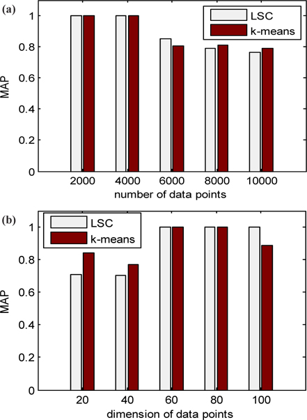
The running time of LSC and k-means for these two datasets is shown in Fig. 4. Figure 4 (a) indicates that the running time of k-means increases much more quickly than LSC when the number of data points increases from 1,000 to 10,000. When the number of data points is at 1,000, the time cost of k-means is at least 100 times more than that of LSC, and when the number of data points increases to 1,000, the time cost of k-means is at least 1,000 times more than that of LSC. Therefore, the advantage of LSC becomes more notable in larger scale datasets. In Fig. 4 (b), we can see the higher the dimensions of the data used is, the more no-table the advantage of LSC is. Even in with low dimension data of 10, the time cost of k-means is at least 10 times more than LSC. To compare the cluster accuracy, MAPs of the two methods were calculated for these two datasets. The results are shown in Fig. 5. The figure indicates that the cluster accuracy of LSC is similar to k-means, and may be better than k-means on some datasets. Therefore, LSC is more suitable for incremental datasets, and it can be a good cluster method for both high dimension and large-scale datasets.

To improve the feasibility of high dimensional data clustering, especially for use in image clustering, an enhanced Locality Sensitive Clustering method based on E²LSH is presented. This method first generates multiple hashing functions, then it projects each point using these hashing functions to get bucket indices. The bucket indices are then clustered to get class labels. In terms of clustering accuracy, experimental results show that LSC’s performance is close to k-means, AP and SC. The advantage of LSC is its fast running speed that makes it suitable for incremental clustering. This property makes it a very valuable method for large dataset clustering and especially for incremental dataset clustering.