Among the different types of transient phase problems, the water-exit phenomenon is one of the less studied and known cases. Prediction of hydrodynamic loads during water-exit of a body is of a great significance in the structural design of marine vehicles. There is no available theoretical tool to completely handle this complicated phenomenon. The water-exit of an initially fully immersed circular cylinder with a constant velocity was first studied by Greenhow and Lin (1983), who have done experimentally and theoretically fundamental studies of non-linear free surface effects. Their physical investigation was based on video recording of the tests. Because of the time-consuming and expensive procedures of the experimental methods in the laboratory, nowadays, Computational Fluid Dynamics (CFD) methods are used widely for handling complicated phenomena and their accuracy in different applications is documented. Colicchio et al. (2009) made some experimental and numerical analysis on a circular cylinder either freely falling on or exiting the water. They used a Navier-stokes solver based on an approximated projection method and Cartesian grid with a level set function scheme for the air-water interface interaction with the solid body. In their experimental work, a detailed measurement of velocity field and the local loads around the cylinder is obtained. In another work, the nonlinear problem of a circular cylinder rising vertically to an interface between liquid media was studied by Gorlov (2000). He considered the nonlinear initial-boundary-value problem in a contour approaching of an interface between two liquid media. Gorlov (2000) presented the perturbations which are generated by a circular cylinder approaching the free surface. Kleefsman et al. (2004) improved VOF method for displacement of free surface. They solved the standard dam breaking problem and also they simulated the drop test of a circular cylinder and a wedge. They presented several snapshots of simulations of a circular cylinder exiting the water and compared it with photographs of experiments. Their visual comparison between simulation and experiment was showed a good agreement.
Qian et al. (2005) used a free-surface capturing method to simulate two fluid flows with moving bodies. They simulated a two-dimensional body emerging from beneath the water surface. They proposed a new scheme in which the normal pressure gradient term splits into hydrostatic and kinematic terms, therefore the gravity source term is exactly balanced by the normal hydrostatic pressure gradient term and no errors will be introduced at the interface with this method of calculating the pressure gradient term. Zhu et al. (2005) made a study on a circular cylinder and free surface interaction using finite difference method on a non-uniform, staggered Cartesian grid. They used a new numerical method called Constrained Interpolation Profile (CIP) by which no sharp interface between air and water is obtained i.e., density changes continuously between the values of air and water densities at the free surface. Lin and Xu (2006) used a computer model for simulation of general turbulent free surface flows. They solved the Reynolds-averaged Navier-Stokes equations and employed the VOF method to track the free surface. They simulated water-exit of a horizontal cylinder in Froude number equal to 0.39 and compared their results with Greenhow results. Lin (2007) used a fixed-grid model for simulation of a moving body in free surface flow. In his model, a body is approximated by Partial Cell Treatment (PCT) and the body motion is tracked by Lagrangian method whereas the fluid motion around the body is solved by Eulerian method. Yang and Stern (2007) studied on a combined-boundary/ghost-fluid sharp interface method for the simulations of 3D two phase flows interacting with moving bodies on fixed Cartesian grids. In the water-exit case, they compared their results with boundary element simulation of Greenhow and Moyo (1997). Another problem is prediction of hydrodynamic slamming loads during water-entry of a body. The slamming force on the step of a flying boat in landing, or the slamming force on the bow of ships is very large and has a great significance. The hydrodynamic force of impact problem (slamming) on seaplanes can damage the structure or lead to hull vibration and cause ship speed reduction.
The water impact problem was first simulated by Von Karman (1929), using the momentum and the water-added mass theory to predict the impact force during the seaplanes landing without the effect of water pile-up during impact. Von Karman made an important assumption that during the initial stages of the impact, the momentum of the water/body system is conserved. Von Karman analysis was refined by Wagner (1931), who had predicted the impact force on the seaplane. Further improvements of this work were proposed by Fabula (1957). Most previous studies on the water impact problem are based on the potential flow assumption. During the past decade some numerical studies were carried out to improve results and overcome the limitations of the traditional analytical approach. Numerical analyses with free surface model by VOF method have been recently conducted by Arai et al. (1994). Nikseresht et al. (2004) have solved the impact problem of a circular cylinder based on viscous incompressible flow. They showed that in the impact problem with the viscous effect the numerical results show better agreement with the experimental data especially in water entry time intervals. Rastegari and Nikseresht (2007) solved the classical problem of water impact of a wedge using finite volume discretization and the VOF scheme for two phase flow. Also they studied the effect of concave and convex curvatures of the wedge on the pressure distribution and the slamming force. Greco et al. (2009) developed an iterative Domain-Decomposition strategy to examine the coupling between the global motions of a Very Large Floating Structure (VLFS) and bottom-slamming events.
In the present paper, numerical simulation of the two and three dimensional buoyancy driven water-exit of a circular cylinder in two-phase flow is made with coupling the rigid body dynamic equations of motion. The two-phase flow is solved based on the finite volume method and the interface is tracked with the VOF scheme. Dynamic equations and a dynamic mesh are used to obtain the real velocity distribution during the water-exit and entry of circular cylinder. Moreover, the oblique exit and entry of a circular cylinder with two exit angles are simulated.
>
Fluid motion & free surface equation
The equations represent a mathematical model for describing viscous flows in the form of Eq. (1) reported by Versteeg and Malalasekera (1995). They are usually called Navier-Stokes equations in honor of two men, the Frenchman M. Navier and the Englishman Stockes, who independently obtained the equations in the first half of the nineteenth century (see Sheikhalishahi et al. (2009)):


The incompressible continuity equation is:

Note that the dynamic condition, i.e., continuity of pressure at the interface is implicitly satisfied. The kinematic condition that the interface is convected with the fluid can be expressed in terms of volume fraction

which is called free surface equation.


where subscript
• Interface tracking methods - Height Function - Line Segment - Arbitrary Lagrangian - Eulerian • Volume tracking methods - Marker And Cell (MAC) - Volume Of Fluid (VOF) - Level Set (LS)
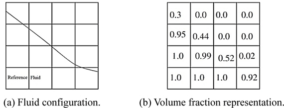
In this research the volume of fluid method is used. The volume of fluid method has been much used for marine hydrodynamics applications. Primarily for internal flows as sloshing in tanks, but it has also lately been applied to external flows problems like flows around ship hulls. This method is a volume tracking technique that was originally introduced by Hirt and Nichols (1981). It can be applied to problems where several fluids with different densities are present. In addition, it can handle complex physical situations such as breaking surfaces, splash, fluid detachment, etc. The main idea of the VOF method is to introduce a function
A typical VOF algorithm generally consists of two parts (see Ransau (2002)): - A device to track the volume and locate the free surface. This device must be able to keep the interface as sharp as possible. - A way to impose boundary conditions at the surface.
The first part of the VOF algorithm, i.e., the location of the free surface consists in a device allowing the accurate computation of the evolution of the function
The dynamic mesh model can be used to model flows where the shape of the domain is changing with time due to the motion on the domain boundaries. The motion can be a prescribed motion, or an un-prescribed motion where the subsequent motion is determined based on the solution at the current time. Three groups of mesh motion methods are available to update the volume mesh in the deforming regions subject to the motion defined at the boundaries:
• Smoothing Methods - Spring-Based Smoothing Methods (SBSM) - Laplacian Smoothing Methods (LSM) - Boundary Layer Smoothing Methods (BLSM) • Dynamic Layering Methods (DLM) • Local Re-meshing Methods (LRM)
In this paper SBSM and DLM are used for dynamic mesh model (see Gessner (2001) and Acikgoz (2007)). In the SBSM, the edges between any two mesh nodes are idealized as a network of interconnected springs. The initial spaces of the edges before any boundary motion constitute the equilibrium state of the mesh. A displacement at a given boundary node will generate a force proportional to the displacement along all the springs connected to the node. The spring-based smoothing is shown in Fig. 2 for a cylindrical cell zone where one end of the cylinder is moving.
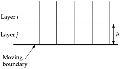
In prismatic (hexahedral and/or wedge) mesh zones, DLM can be used to add or remove layers of cells adjacent to a moving boundary, based on the height of the layer adjacent to the moving surface. The layer of cells adjacent to the moving boundary is split or merged with the layer of cells next to it (layer
LRM is useful when the boundary displacement is large compared to the local cell sizes, the cell quality can deteriorate or the cells can degenerate.
Dynamic equations of solid body motion in the inertial coordinate system are as follows:


where is the force (
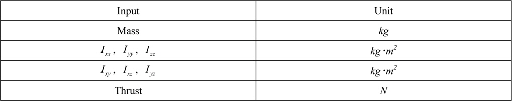
[Table 1] Input data for motion description.

Input data for motion description.
So the linear and angular accelerations of the body are obtained from Eqs. (7) and (8). Integrating acceleration, the linear velocity


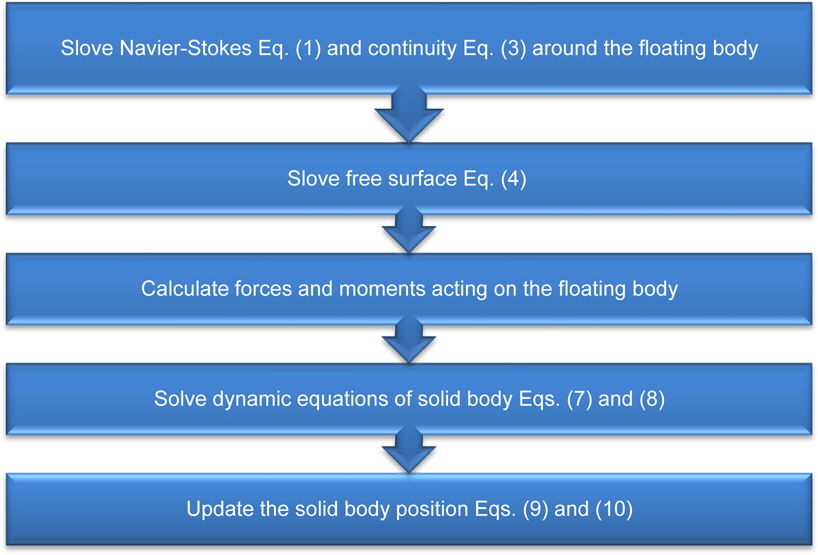
Fig. 4 shows the numerical algorithm for rigid body motion simulation. As it is depicted in Fig. 4 at each time step the Navier-Stokes and continuity equations around the floating body are solved and the interface is tracked with the VOF scheme and forces and moments acting on the floating body are calculated. So by solving dynamic equations of solid body motion, the new position of the cylinder is achieved.
>
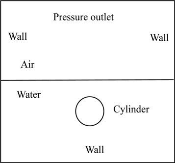
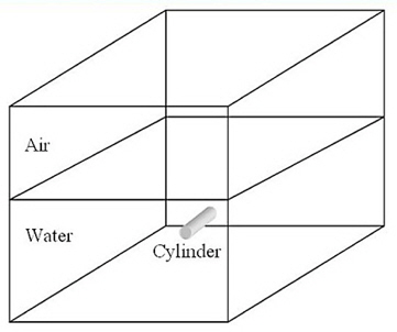
Problem domain and boundary condition
A cylinder with weight equal to 0.62 times the weight of the water and diameter of 30
Fig. 6 shows the transition between adjacent cell zones and the dynamic layering cell zone.
The Weber number is a dimensionless number in fluid mechanics that is often useful in analyzing fluid flows where there is an interface between two different fluids, especially for multiphase flows with strongly curved surfaces. It can be thought of as a measure of the relative importance of the fluid's inertia compared to its surface tension. Water has a high surface tension of σ = 0.0727
>
Parallel processing for 3D simulation
In parallel processing, according to the number of the processors that are used in the calculation, the domain has been decomposed to several sub-domains. In order to obtain a good load balance, each sub-domain must contain the suitable number of cells (see Sheikhalishahi et al. (2009)). Speedup of calculations by increasing the number of processors is an important problem in parallel processing. More details about parallel processing and partitioning in different kinds of mesh domains can be found in Schiffermuller et al. (1998). Specifications of Hybrid Cluster which is used in 3D simulation are listed in Table 2.
[Table 2] Specification of hybrid cluster.

Specification of hybrid cluster.
Water exit results of a circular cylinder are presented in four parts. At first, a cylinder rising only due to its buoyancy is simulated and the results are compared with other numerical and experimental data available in the literature in order to validate the numerical method used in this research. The conditions of this simulation are noted as Test No. 1 in Table 3. In this case no thrust is exerted to the cylinder.
In the second part, the effect of cylinder mass is investigated for the Test cases 2 to 5 described in Table 3. In these cases an external vertical force is added such that the net vertical (body and external) force remains unchanged. The third part of the results shows the applicability of the present numerical method in modeling other complicated phenomena. In this part, waterexit of a circular cylinder with the path angle of 30° and 45° is simulated. For this purpose an external horizontal force is added to the Test case No. 4 such that the net resulting force vector makes an angle of 30° or 45° with the vertical direction. More details are shown in Table 4.
[Table 3] Parameters of the water-exit simulations.
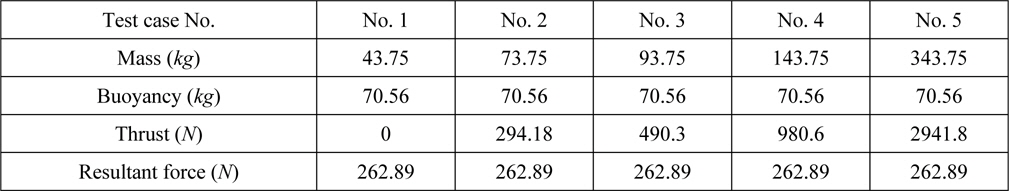
Parameters of the water-exit simulations.
[Table 4] Parameters of the oblique water-exit simulations.
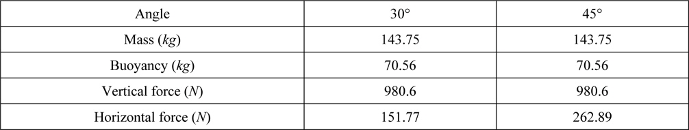
Parameters of the oblique water-exit simulations.
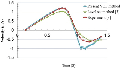
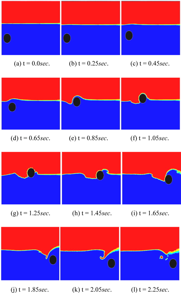
In the first simulation (Test No. 1), buoyancy force causes the upward motion of the circular cylinder. The free surface will deform continuously till the cylinder exits completely. During the exit of the cylinder, a thin water layer around the cylinder is lifted. By further raising the cylinder up, the water layers in the circumference of the cylinder are drawn down to the water surface and cause the breaking of the free surface. This phenomenon takes near 1.0
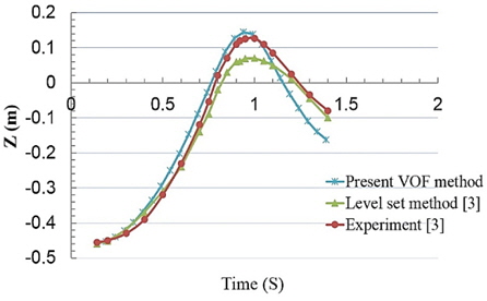
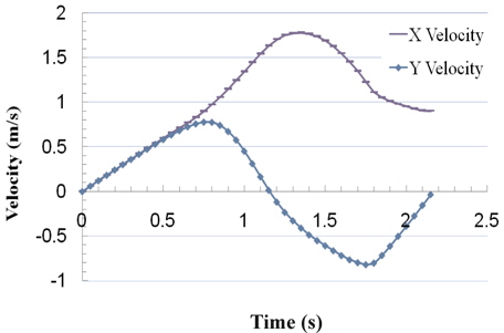
Fig. 8 shows the cylinder center position during water-exit. As it is shown in these figures, the results of the present simulation method predict the velocity and position of the cylinder with high precision during water-exit when they are compared with experimental data.
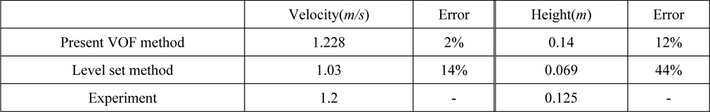
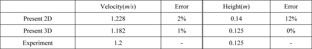
It should be noted that the simulation error of the present work for maximum velocity and height in Figs. 7 and Figs. 8 is about 2% and 12% respectively (see Table 5), while the corresponding errors of Colicchio et al. (2009) level set method are about 14% and 44%. It should be noted that Colicchio et al. (2009) used a two phase Navier-Stokes solver based on approximated projection method and the equations are discretized on a Cartesian staggered grid with a second order approximation both in time and space.
[Table 5] Maximum velocity and height during the water-exit.

Maximum velocity and height during the water-exit.
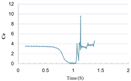
So it can be concluded that in water-exit problems, the present VOF method is more accurate than the Colicchio et al. (2009) numerical level set model which is described above. However the present simulation has less precision in water reentering phase due to the free surface deformation shape, just below the cylinder. The non-dimensional exit coefficient


where
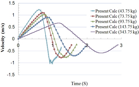
In Test No. 2 as it is shown in Table 3, the forces that act on the cylinder are thrust plus buoyancy force. Also the mass changes so that the total force remains constant like Test No. 1. Therefore in Eq. (7) the total force F remains constant and the mass is increased and so the acceleration is decreased. It causes the velocity and position of the cylinder to change. It can be repeated with various masses in test cases 3, 4, and 5. Fig. 10 shows the time variation of the velocity for different masses. As it shows, increasing the mass reduces the pick value of velocity because of greater inertia.
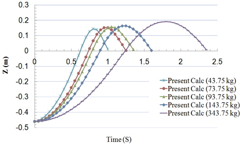
The effect of different masses on the position of the center of the cylinder is plotted in Fig. 11. It is apparent that increasing the mass delays the exit time of the cylinder from the water surface, but the cylinder goes more up in the air.
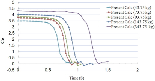
Fig. 12 shows the variation of exit coefficient for Test No. 1, 2, 3, 4 and 5. Similar to the position diagram, the exit coefficient increases with the increase of the mass.
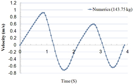
Fig. 13 shows the variation of the velocity for Test No. 4 in two cycles of exit and again entry phases of the cylinder. The maximum pick of the velocity is decreased due to the effect of the hydrodynamic force in the exit and entry phases. It will continue until the cylinder reaches the zero velocity and gets a static condition. The variation of the velocity of the cylinder generates waves from the cylinder on the free surface.
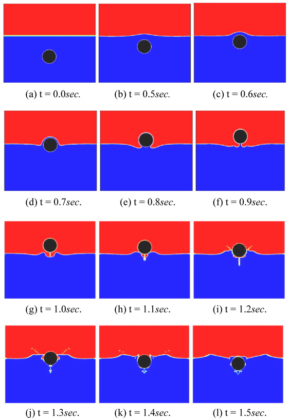
The time evolution of the free surface for Test No. 2 is illustrated by density function in Fig. 14. After the cylinder exited the water and again dropped into the deformed free surface at t = 1.1
In order to show the applicability of the present method for modeling other complicated phenomena, water-exit of a circular cylinder with the path angle of 30° and 45° is carried out. More details are shown in Table 4. After releasing the cylinder, with an acting vertical force equal to 980.6N and an acting horizontal force equal to 151.77
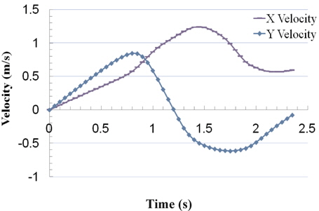
When the cylinder starts its motion to exit, horizontal and vertical velocity of the cylinder increase gradually. As it is depicted in Fig. 17, when the cylinder with the path angle of 30° reaches the water surface, the effect of buoyancy force is quickly removed and it causes a decrease in vertical velocity. But due to the decrease of water resistance, the horizontal velocity is still increased with greater acceleration until it again impacts on the water at time = 1.45
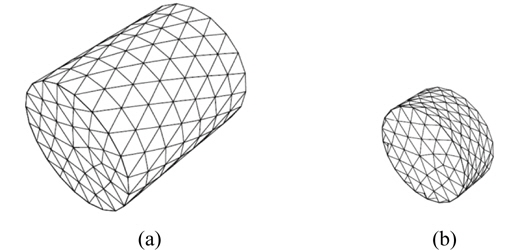
A cylinder with weight equal to 0.62 times the weight of the water and diameter of 30
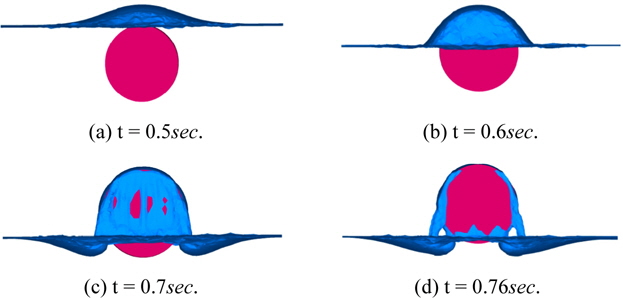
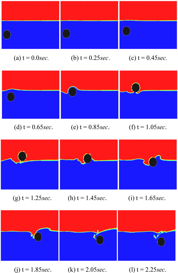
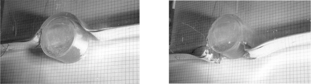
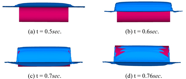
In the 3D simulation, buoyancy force causes the upward motion of the circular cylinder. Fig. 20 shows exit of the cylinder for various times in x-z plane, the water above the cylinder is lifted with the cylinder and forms a thin layer of water on the cylinder. As it is shown in Fig. 20 (t = 0.6) the fluid particles at the free surface on the cylinder are lifted by the cylinder and then fall away rapidly from the cylinder (t = 0.7). This phenomenon is also seen in experiments which were reported by Kleefsman et al. (2004) (Fig. 21). By further raising the cylinder, the water layers in the circumference of the cylinder are drawn down to the water surface and cause the breaking of the free surface. Afterwards the cylinder falls down again because of its weight.
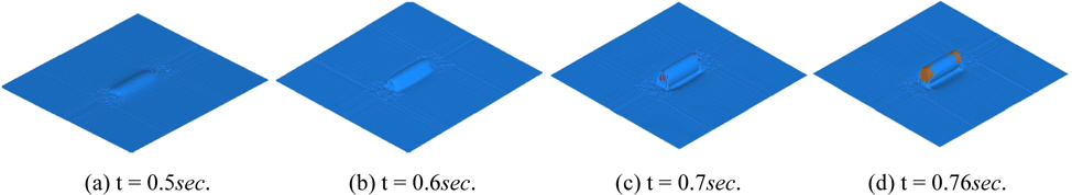
In Fig. 22, the non-linear free surface deformation in water-exit of a circular cylinder in y-z plane is shown. Fig. 23 shows the numerical simulation of water-exit of the circular cylinder in 3D view. One of the aspects of 3D simulation in comparison with 2D simulation is the visualization of water flow on the top surface of the cylinder and the free surface breaking on the front and back faces of the cylinder in the exit phase in 3D simulation, which cannot be seen in 2D simulation.
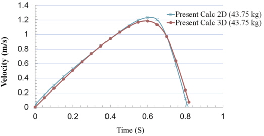
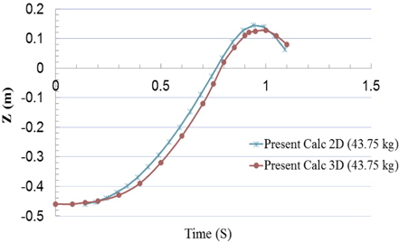
Fig. 24 shows the comparison of cylinder center velocity in 2D and 3D simulations. As it is depicted in this figure and Table 6, the maximum exit velocities which are predicted in 2D and 3D simulations are in a good agreement with each other and experiment, but, it should be noted that the error in the position of the cylinder in 2D and 3D simulations with respect to the experimental data is near 12% and 0% as it is shown in Fig. 25 and Table 6. This confirms the ability of the present 3D numerical method (VOF method) to predict accurately the water-exit velocity of a circular cylinder. As it is depicted in Fig. 26 in the water-exit phase, the cylinder drag force on 3D simulation is a little higher than 2D one, because of the additional front and back faces of the 3D cylinder. So the velocity in 3D case increases at a lower rate and finally cylinder travels a lower distance at the same time in comparison with 2D cylinder motion.
[Table 6] Maximum velocity and height during the water-exit in 2D and 3D simulations.
Maximum velocity and height during the water-exit in 2D and 3D simulations.
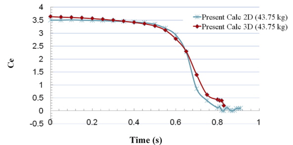
Fig. 26 shows the variation of the exit coefficient in 2D and 3D simulations. The exit coefficients also in 2D and 3D simulations are in a good agreement and have only a few differences. This small difference may be due to the effect of the downwards water in two ends of the cylinder that cannot be predicted in 2D simulation. The trends of exit coefficient which are predicted in 2D and 3D simulations are the same. So if one only needs to use the exit coefficient of the cylinder and does not want to analyze and observe the details of the water exit phenomena it is recommended to use 2D simulation instead of 3D.
This paper presents a numerical simulation of water-exit of a circular cylinder using the equation of solid body motion. The finite volume method is used to solve the Navier-Stokes equations. Volume tracking method VOF is used for simulation of free surface deformation during the water-exit of the circular cylinder. For calculating the effect of the velocity change, dynamic mesh method is used. The present simulation shows an excellent agreement with experimental data in water-exit phase and also in its motion outside water before impacting the free surface. This numerical method, based on VOF model is more accurate than level set model used in another numerical simulation.
The velocity and motion of the cylinder in water-exit simulation agrees well with the numerical results of Colicchio et al. (2009). The complicated free surface deformation is simulated having a good agreement with the experimental results of Kleefsman et al. (2004). Furthermore, the effects of changing mass and thrust with superposition of the buoyancy force with the limitation of having a constant total force is simulated. The numerical results show the applicability of the present method for modeling complicated phenomena. After investigation of mass effects, oblique exit of a circular cylinder for two exit angles is simulated. Then using parallel processing, water-exit of the circular cylinder in 3D is simulated and compared with 2D simulation. The results of 2D and 3D simulatons showed a good agreement. The strongly non-linear free surface deformation in waterexit of a circular cylinder is simulated successfully with an excellent agreement with the experiments.