If we want to analyze the motion of a body in a fluid, we should analyze the rigid-body dynamics of the body and the fluid dynamics of the surrounding fluid. Traditionally, the potential theory has been used for the analysis of the flow of fluid in studying the motion of ships. Added mass, which is the mass of surrounding fluid moving together with a ship, was treated as part of the virtual mass of that ship, and the wave damping forces were treated as the damping of the body. The main external force comes from incident waves, so gravity wave dynamics had to be solved, and the resultant pressure was integrated over the body surface to form the wave external force.

Currently, in analyzing ship motion, besides the potential theory, Computational Fluid Dynamics (CFD) based on the Navier-Stokes equation is being used; owing to the development of computers. One of the main differences between the potential theory and CFD is the treatment of added mass. In the potential theory, the added mass can be expressed explicitly, so one obtains the added mass, adds this to the mass of the ship, and then analyzes the ship motion. However using CFD, the ship motion analysis is done by first solving the flow of surrounding fluid for a given ship motion; then adding the pressure forces acting on the ship surface into the external forces of the equation of motion. This is because the inertia forces due to added mass cannot be expressed explicitly, so one cannot help but treat it as external force. Thus the difference is whether the added mass can be treated as ship-mass or be included in external forces. Using CFD, an assumption of convergence is made; that is, there is no problem if the time interval for time integration is reduced sufficiently, even if the inertia force due to added mass is treated as external force.

In this study, we revisited the property of added mass, investigated its property in the equation of motion, and the problems that can take place. Our work revealed that the equation of motion has a self-similar structure if the forces due to added mass are treated as external forces; then the solution can diverge. In differential equation, the highest order differential term has the most important role in the equation. We say that the equation has a self-similarity, if the variable to be sought(the highest order differential term) is expressed by forcing terms including that variable itself. In a numerical example, it was shown that the solution can be divergent even if the time interval is reduced sufficiently. This divergent solution may be a false solution due to the self-similarity of the equation, not due to the dynamic property. When using the non-linear potential theory or CFD based on the Navier-Stokes equation for analysis of the surrounding fluid, the reconfiguration technique using ‘pseudo-added-mass’ to resolve the problem of self-similar structure was proposed. The pseudo-added-mass is indeed mass that is pseudo-added in order to ensure a convergence of the solution.

The concept of added mass or virtual mass has appeared in the literature since 1828, when Friedrich Bessel described the motion of a pendulum in fluid domain. The period was longer than that in the air, and this phenomenon was explained as being due to an increase in the effective mass by the surrounding fluid. Later, the concept of added mass played an important role in the analysis of the motion of a body, and the added mass was obtained analytically for simple shapes. Surely, the concept of added mass has been used in ship motion analysis, but the added mass could only be obtained after the shape of the ship was modified to a less accurate, simpler shape.

The added mass of more ship-like shapes was obtained by Lewis (1929). He used the conformal mapping technique to mathematically represent the shape of the ship cross section; a result that is now called the Lewis form. He used added mass in his analysis of the vibration of a ship. Hess and Smith (1962) proposed the numerical method to calculate the potential flow around a 3-dimensional body of arbitrary shape. The added mass of a body floating on a free surface has different characteristics from those of a body in unbounded fluid. The formulations on this problem were made by Ursell (1949), and John (1949; 1950). Ursell (1949) analyzed the motion of a circular cylinder on a free surface by obtaining the added mass using the multi-pole expansion method. Later, Tasai (1959) developed the multi-pole expansion method further to obtain the added mass of a Lewis form on a free surface. Now, the added mass of ship-like section could be calculated. Frank (1967) proposed a calculation method for added mass of an arbitrary shape, and more developments on this method made it applicable to 3-dimensional shapes. Newman (1978) gave a good account of the history and efforts toward representing the motion of a ship.

In order to describe the motion of a body in the fluid domain, the two systems of dynamics are needed: rigid-body and fluid dynamics. For convenience, the explanation will be given for a 1-dimensional problem, but this logic can be applied to 2 and 3-dimensional problems as well. According to rigid-body dynamics, Newton’s law appears in the form:

where m is the mass of a body, and v, x are the velocity and position of the body, respectively. If we assume that the mass of the body will not alter in time, the equation becomes:

If we suppose that the body is in the fluid domain, the force in the above equation includes the forces due to the pressure of fluid and other forces f ′ ; such that:

This equation has the meaning that we can calculate the motion of the body if we know the forces acting on the body (the right hand side terms of the equation). The forces acting on the body could be obtained by solving the fluid pressure for a given boundary condition, which represents the velocity component on the body surface due to the movement of it. There seems to be no contradiction in the formulation. Let us consider another way to formulate this problem. In an ideal fluid, the energy of the fluid when a body moves in it can be expressed as follows (Landau and Lifshitz, 1959):

E = mikuiuk

where m_ik is the induced-mass tensor, and u_i is the velocity component. In the above expression, the repeated index means summation over the motion-mode according to tensor notation. The induced-mass is the coefficient of the term of velocity squared; resulted after the fluid energy is integrated over the entire domain and rearranged by order of velocities. In one dimension, this can be represented as Once the energy of the fluid is known, the momentum of the fluid can be described as dE = v ⋅dP . Consider the system in which the body and fluid are included together. The equation of motion of this system can be derived, representing the force by the time rate of the momentum of the system as:

If we represent the fluid momentum by fluid energy, the equation of motion can be reduced to

Comparing Eq. (5) with Eq. (3), we can see that the mass in the equation of motion is altered from body mass to virtual mass. In order to investigate the difference in the two equations, let us see how the integration of pressure on the body surface can be represented in potential theory. Newman (1977) gave the result of the expression of pressure force in potential theory as follows:

where ϕ^x is the velocity potential of flow when the velocity of the body is a unit in x-direction. Substituting Eq. (6) into Eq. (3) results in

The two equations Eqs. (5) and (7) in an ideal fluid have only one difference between them. That is the position of the inertia force due to added mass in the equation of motion. Fortunately, this difference can be shown because of the explicit expression of added mass in potential theory. Even if the force due to added mass cannot be expressed explicitly as in Eq. (6), Eqs. (3) and (7) show that the force due to it will be included implicitly in the right hand side of the equation as external force; if the force due to pressure integration is treated as external force as in Eq. (3). Eq. (7) (derived from Eq. (3)) is the result from matching rigid-body dynamics and fluid dynamics; while Eq. (5) is derived for the system of body-fluid. There is only one difference between them; however, the meanings of the two equations are quite different. In Eqs. (3) and (7), the terms on the right hand side should be known or given. Suppose the current time is t, the right hand side terms should be interpreted as values at the time t⁻ , which is the time infinitesimally earlier than t. Let us integrate Eq. (7) for the interval ( t,t + h ) such that:

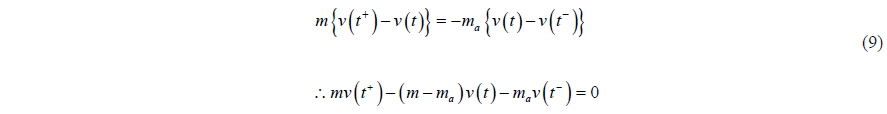
Taking the limit of h to 0, the above equation results in

where t⁺ is the time infinitesimally later than t. In order to see the stability of the above equation, let us introduce the growth factor, the ratio of the values of the same variable at t⁺ and t, or t and t⁻ such that:

β = v (t+ ) / v (t) or β = v (t ) / v (t− )

The characteristic equation of Eq. (9) using the above growth factor and the solution of it are:

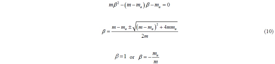
If the absolute value of growth factor β is less than or equal to 1, the solution does not diverge, but the solution becomes divergent if the added mass is greater than the mass of body. The fact that should be noticed is that this phenomenon takes place even if the time interval h is decreased to zero. This is the inherent problem. If the above is correct, the body cannot move in the fluid, or diverges instantaneously if the body starts to move in the fluid; when the added mass is greater than the body mass. Thus Eqs. (3) and (7) seem not to be adequate for the description of the motion of a body in a fluid. The reason is that Eq. (7) has self-similar structure because the physical variable that is sought ( ), appears on the right hand side of the equation. The problem of divergent self-similar structure should be resolved by the renormalization technique in order to represent physical phenomena properly (Parker, 1983). The equation of motion that can better represent the motion of a body in a fluid is Eq. (5).

Comparing this with Eq. (3), the mass in the equation is altered, that is, the structure of the equation is different. In this case, does Eq. (3) present any problems? Even if the two systems of rigid-body and fluid dynamics have no problems, and are self-consistent, the coupled system may have self-similar structure when the two systems interact with each other. That is to say, even though the equations here seem to be perfect in each sense, problems may arise in the system in which the components interact with each other. In the case of differential equations in which the highest order terms appear on both sides, the equation should be modified so that the highest order term can appear only on the left hand side.

In summary, the force due to added mass originally comes from the surrounding fluid, but should be included in the mass term of the equation of motion because it is proportional to the acceleration of the body. The concept of added mass is often called the first example of renormalization in physics. In potential theory, the force due to added mass can be expressed explicitly as the product of the added mass and the acceleration of the body. But when the fluid dynamics is analyzed using CFD based on the Navier-Stokes equation, the force due to the fluid pressure also includes the effect of added mass, even though it cannot be expressed explicitly. Thus, the structure of the equation of motion becomes self-similar.

Let us consider the equation of motion relating to the added mass. The focus is on how the fluid force is represented, and on the concept of the treatment of added mass; not on the details of the equation of motion.

The linear theory for analyzing the motion of a body was developed mainly with the potential theory. There are two main streams of analysis: one for the frequency-domain and the other for the time-domain. The two results are related to each other through a Fourier transform because of their linearity. Let us see a method for expressing the fluid force.

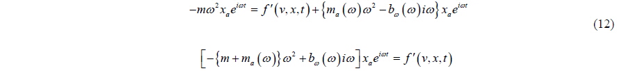
In frequency-domain analysis, only the time-harmonic terms are considered; not the transition terms. The hydrodynamic force can be expressed as:

The equation of motion can be represented as:

The added mass is expressed explicitly in the fluid force expression, so the added mass term can be moved to the left hand side of the equation. Because of the existence of a free surface, the added mass is dependent on the frequency; which means that the added mass varies in time.

In time-domain analysis, the impulse-response function is used. It is defined as the time history of the fluid force when the velocity of the body is given as impulse.

where A(ω) , B(ω) are the added mass and wave damping coefficient, δ is the Dirac delta function, and δ′ is the time derivative of the Dirac delta function. The wave damping coefficient is integrable because its value is finite and tends to zero at infinity. Using the impulse-response function, the fluid force can be written as:

where

Substituting Eq. (14) into the equation of motion results in:

Moving the term proportional to acceleration to the left hand side:

The motion of the body can now be calculated without any problem using Eq. (16), which has been reconfigured by renormalization.

If there is no free surface, the fluid flow has linear properties, while the pressure has non-linear terms. However, the flow of fluid has non-linearity if a free surface exists. Using potential theory, the pressure force can be expressed as:

where n_i is the component of normal vector in the direction of the motion mode. If the free surface and body surface are tracked by the semi Euler-Lagrangian scheme (Longuet-Higgins and Cokelet, 1976), the pressure on the surface should be represented by a substantial derivative.

It is impossible to extract the added mass explicitly from Eq. (18).

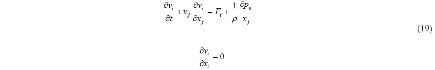
Let us consider the equation of motion, in which the external force is represented by using the flow from the Navier-Stokes equation. First let us check whether the added mass is included in the pressure force, or not. Although we are hear considering one dimensional flow, the result can be expanded to 2 and 3-dimensional flow without loss of consistency. The Navier-Stokes equation and continuity equation are:

The momentum equation becomes the Euler equation for a non-viscous fluid.

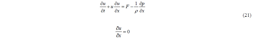
For one dimensional flow, Eq. (19) can be rewritten as:

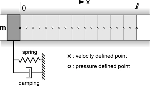
Let us consider the simple problem shown in Fig. 1, in which the body is located at x = 0 , and fluid occupies the region( 0 < x < l ). Assume that the fluid can move only in the x-direction, the viscous effect is neglected, and that the pressure vanishes at x = l .

The boundary condition is the same as the velocity of the body. The pressure for the above example can be obtained easily as:

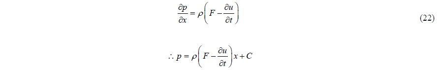
Applying the pressure condition, we can obtain the pressure.

The pressure at x = 0 acts on the body surface, and the force can be obtained as follows:

Eq. (24) shows that the fluid mass is the added mass and the fluid force is explicitly proportional to the body acceleration. This means that the pressure force includes the force due to the added mass. For a 1-dimensional case, the explicit expression of added mass in the force can be obtained, but for 2 and 3-dimentional cases, it may be impossible to get that type of expression. The important thing to notice is that the pressure force includes the force due to the added mass, no matter whether the expression is explicit or implicit.

Let us consider what happens if we solve the above problem numerically. We use the acronym for Semi-Implicit Method for Pressure Linked Equations (SIMPLE) (Patankar, 1980) algorithm to solve the incompressible Navier-Stokes equation. The numerical procedure generally follows the following steps. The fluid region is divided into a number of grids and cells. The pressures at the center of cells are defined, as is the velocity at the mid-point of the grids. Assume the velocity u at time step n −1 is correct. At time step n , the change in the velocity of the body from uⁿ⁻¹ to uⁿ compresses the first cell and the pressure in the first cell increases. Then the velocity, defined at the middle of the first and second cells accelerates. This change of velocity compresses the next cell, and accelerates the neighboring velocities, and so on. The pressure can then be obtained by iterating the above calculation until all cells satisfy the continuity equation (second equation of Eq. (21)). The resulting pressure becomes:

The pressure obtained above is proportional to the velocity difference in time, and it can be interpreted as the value at time step n−1/ 2 . The pressure force on the body surface is:

where m_f = ρl is the mass of fluid that moves with the body, that is, the added mass. Eq. (26) is the numerical version of Eq. (24). This means that we will obtain the same result independent of whether the problem is solved analytically or numerically. That is, the pressure force includes the force due to added mass, and the point of difference is that this value is now interpreted as the value at the time step n−1/ 2 .

If we neglect the spring in Fig. 1, the equation of motion can be written as:

If we specify the time of definition to each terms of Eq. (27), in the strict sense,

Shifting the time backward by h / 2 makes the equation:

This equation shows that the force due to added mass will be included in the external forces, and that the time definition of it is t − h (i.e., the previous time step), if we solve the problem by obtaining the pressure force from fluid dynamics and put it into the external forces of the equation; not directly obtaining the added mass. Two facts make problems in the equation of motion. One is that the acceleration on the right hand side is defined as that at the previous time step. The other is that the force due to the added mass is treated as an external force, while it is the highest order term in the equation. It is tempting to think that the smaller time step will remove all the problems; however, as seen in the previous section, the problem cannot be resolved even if the time is zero. This is inevitable because the highest order term is treated as an external force in the above equation. That is the self-similarity problem in terms of mathematics and physics.

In order to investigate conceptually the problem of the added mass, let us simplify the problem to include the important terms only. Dividing Eq. (5) by the virtual mass (sum of the mass and added mass), and simplifying the system forces to include only damping force leads to:

The characteristics of the equation are included in the homogeneous equation.

The solution of the above equation is stable no matter what method is used. The solution may be obtained analytically as:

If the fluid force is expressed using non-linear potential theory, or the Navier-Stokes equation, the equation of motion has a structure like Eq. (3), and the force due to the added mass is included on the right hand side of the equation. Here we modify Eq. (30) to that structure.

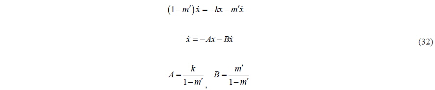
where m′ is the ratio of the added mass and the virtual mass. The structure of Eq. (32) is similar to that of successive substitution. This is because the equation has a self-similar structure. Let us specify the time stamp on the variables, and integrate the equation using the Euler method such that:

Modifying the above equation gives:

In order to have only x terms, and not the derivatives, in the equation; let us change the last term in Eq. (34) such that:

Next, then the growth factor β can be obtained by:

For a small h, the growth factor becomes:

The growth factor β₁ is always less than 1, but β₂ is directly dependent on B. The important point is that if B is greater than 1, the absolute value of β₂ is always greater than 1; even though the time step h decreases to zero. Therefore, instability will take place if B is greater than 1. Furthermore, once a small error exists, at one time it will be greater than the exact solution, and at the next time it will be smaller than the exact solution. That is to say, the error will bounce back and forth around the exact solution and grow in magnitude for each step. Thus, the region of stability becomes:

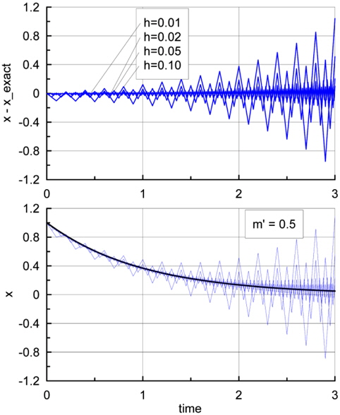
In other words, we can obtain a stable solution from the equation of motion only if the added mass is less than the mass of the body. The above criterion for numerical stability agrees well with that for the theoretical one (Eq. (10)). This means that if the condition in Eq. (38) is not satisfied, we will obtain divergent solutions no matter what the numerical scheme is (even using Runge-Kutta or higher order methods). Furthermore, it is clear that the same problem will arise in a second-order differential equation in which restoring force exists.

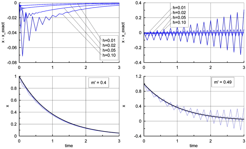
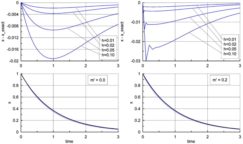
In order to see how the numerical solutions appear in real numerical calculations, some numerical calculations for the same virtual mass were done and the results were illustrated in Fig. 2 through 4. For convenience, the chosen value of k was 1, and the time steps 0.01, 0.02, 0.05, and 0.1.

The ratio m′ can be interpreted as the amount of mass which is treated as the external forces in the right hand side of the equation. Because all the results are for the same virtual mass, it is easy to compare the effects of that portion of the virtual mass which plays the role of external force when the equation has a structure like Eq. (3). Fig. 2 shows the result when m′ is 0.0 and 0.2 (i.e., when all the virtual mass is treated as the system inertial mass and a 20% portion of the mass is treated as the external force). As expected, the numerical solution goes toward the exact solution as the time step size decreases. When m′ = 0.2 , there exists a short oscillation in the initial period. When m′ increases to 0.4, the oscillation grows in magnitude and is sustained for a longer period of time, as shown in Fig. 3. The oscillation is not the oscillation of the dynamic system; it is a false solution and bounces back and forth. When m′ = 0.49 , the small time steps make the absolute value of β₂ less than 1, and the large time steps make it larger than 1, so the solution with large time steps diverges, while that with small time steps converges. When m′ = 0.5 , the limit of stability, all numerical solutions diverge regardless of the time step size. With these results, it was shown that the instability of the equation, in which the force due to added mass is treated as external force, must arise not only in theory, but also in numerical calculation.

As seen in the previous sections, we know that the equation of motion should be solved after modifying the equation via the renormalization concept(i.e., so that all the inertia forces appear in the left hand side of equation of motion), when the added mass which is included on the right hand side of the equation is greater than the mass of a body. When the added mass is less than the mass of a body, for example the motion of a deep buoy, there is no big difficulty in calculation of motion except for the bouncing transition solution of the initial stage. However, in the case of the heave and pitch of a shallow draft ship, an instability problem may arise because of a large amount of added mass and moment of inertia. This conclusion can be applied to rotational motion. For the roll of a ship, the added moment of inertia of fluid is usually less than that of the ship, so the solution may be obtained without great difficulty.

In cases where all the pressure forces are treated as external forces like Eq. (3) (i.e. using non-linear potential theory or the Navier-Stokes equation), the stability problem may arise. This is particularly true when the added mass is greater than, or equal to, the mass of a body. This is because the equation of motion has a self-similar structure. To resolve this stability problem, all one has to do is move the added mass term to the left hand side of the equation when the added mass term is expressed explicitly. However, when the added mass cannot be expressed explicitly, one may add the same quantity to both sides to resolve the problem. Here we introduce a method for adding ‘pseudo-added-mass’.

where [m_a] is the pseudo-added-mass. This ‘pseudo-added-mass’ is indeed mass that is pseudo-added in order to ensure a convergence of the solution. It may be defined so that it satisfies the stability condition if the added mass is not known. The best way to define it is using the added mass in an unbounded fluid, or that of infinite frequency. The stability criterion is as follows:

In cases that there is no choice but to put the force due to the added mass on the right hand side of the equation, reconfiguration by adding the ‘pseudo-added-mass’ can resolve the self-similar structure of the equation of motion.

The rigid-body dynamics and fluid dynamics of a fluid surrounding a body are self-consistent and seem to be exact. However, when the two dynamics are coupled with each other in order to produce the equation of motion, the resulting equation of motion may have a self-similar structure. Furthermore, when the added mass is greater than the mass of a body, the solution of that equation will diverge instantaneously, and this problem is shown to be inherent.

This study reviewed the structure of various types of equation of motion. The equations using the traditional potential theory resolve this problem of self-similarity by introducing the concept of the added mass, but equations using a non-linear potential or the Navier-Stokes equation have a self-similar structure.

In order to see whether the inherent problem of self-similarity happens only in theory, a numerical study was done. The results showed that the numerical solutions also have the same property as theory, except for the effect of time step size.

With the results obtained in this study, a reconfiguration method using ‘pseudo-added-mass’ was proposed. It may be useful for resolving the divergent phenomenon caused by self-similarity when the implicit added mass is greater than the mass of a body.

In this study, the analysis involved a 1-dimensional case, but its logic can easily be applied to 2 and 3-dimensinal cases. The author hopes that provisions for 2 and 3-dimensional cases will be made in the future.