Wave run-up over coastal structures and breakwaters is one of the most important hydraulic reactions used in crest elevation of designs for coastal structures. The design of rubble mound breakwaters is typically based on empirical formula and physical modeling. One limitation of this approach is that there are many different aspects of wave interaction with a breakwater, such as elevation of the run-up tip and armour stability and these are treated separately. Nowadays the development and evaluation of numerical models to simulate run-up phenomenon is one of the most interesting topics in coastal engineering.
Numerical models are useful tools applied to the early design stages of coastal structures, they are used to help coastal physical modeling in the design tests to measure quantities that are difficult to assess in other modeling techniques such as prototype and scaled down physical models (Altomare et al., 2012). Until recently, numerical models could not predict the complex wave situations that occur in front of breakwaters. So far, wave runup and overtopping on rubble mound breakwaters have been investigated by many researchers (Van Der Meer et al., 2005).
There are two viewpoints for investigating the interaction between fluid and structure: the first supposes that a porous medium has no effect on characteristics and flow pattern and as such a structure's geometry is modeled according to a solid object with a porosity value. In such cases, calculations made out of a simple assumption do not work well in evaluating flows with high Reynolds and in cases when a breakwater constitutes large pieces such as concrete armour pieces. In the second viewpoint, porous medium geometry is modeled precisely and in such cases, fluid can move inside a porous solid object (Dentale et al., 2012). The second model obviously requires fabricating a shape's complex geometry and applies more computational cells, but it provides a more accurate model. Dentale et al. (2009) introduced an innovative RANS/VOF procedure by integrating CAD and CFD software to analyze the hydrodynamic aspects of the interactions between breakwaters and waves. Their method produced better results than the traditional approach whereby the flow within the armour is computed with seepage flow approximation (Cavallaro et al., 2012). Latham et al. (2008) used discrete element and combined finitediscrete element methods to model the granular solid skeleton of randomly packed units coupled to a CFD code which resolves the wave dynamics through in interface tracking technique. Latham et al. (Latham et al.2008; Latham et al.2013) and Xiang et al. (2012) demonstrated that FEMDEM provides excellent shape representation and deformability for static and dynamic problems for faceted and angular concrete units and rock blocks used in armour layers. Their method also provides a powerful tool for examining stress chains within granular packs of armour units.
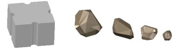
This present research work investigates the wave run-up on breakwaters covered by antifer units via Flow-3D and Auto-CAD software, and is supported by the second mentioned viewpoint that incorporates an accurate geometric model of the breakwater. AutoCAD is utilized to construct different parts of the breakwater's geometry such as core, toe and armor layers. In Fig. 1, armour and other used stones into the stone layer and the breakwater's toe are also shown.
RANS type RNG model is used for the turbulence modeling. The numerical results obtained by Bakhtyar et al. (2010) revealed that the RNG turbulence model yielded better predictions of nearshore zone hydrodynamics, although the k-ε model gave satisfactory predictions.
Flow-3D is the computed fluids dynamic model in this research work. The software is capable of considering different boundary conditions of fluid and to solve the common interface of fluid with fluid and fluid with air. Proposed model is utilized in different applications of hydraulic engineering and coasts such as flow and erosion around hydraulic structures and transmission of waves near the beach. Flow-3D solves three-dimensional Navier-Stokes equations and continuity equation simultaneously. The flow is described by the general Navier-Stokes equations (Dentale et al., 2012):


where
Flow-3D is a non-hydrostatic model. Non-hydrostatic models do not apply simple assumptions into momentum equations, so these must be solved repeatedly. Flow-3D uses a method that considers ‘volume of fluid’ (VOF) to study the common interface of fluid with air and fluid with fluid. This method records levels of fluid volume for each cell. This volume is then used to determine comparisons with evaluations for cell adjutant volumes for ant, slope, position and curvature of the fluid into cell. Rigid boundaries are simulated by means of the
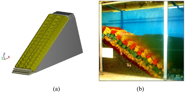
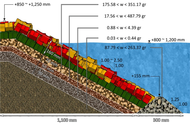
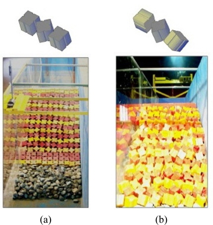
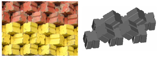
Experimental data of modeling a breakwater's hydraulics (by Najafi-Jilani and Monshizadeh, 2010) in Pars petrochemical port (in Iran) were used to calibrate and verify the numerical model. Physical modeling was carried out by using a geometrically undistorted 1:22.5 scale with respect to the prototype and by guaranteeing Froude similarity. Virtual models of the breakwater was built as same as experimental model dimension (see Figs. 2 and 3). The wave flume was 25 meters in length, 1 meter in width and 2.5 meters high. Virtual model of the breakwater is constructed according to an experimental model to verify the software so that it has more compatibility with a real structure. Fig. 2 indicates a view of the breakwater in lab flume and positions of its layers of core (first layer), filter (second layer a), under layer (second layer), stone layer (third layer) and stone toe (third layer a). The stone layer was covered by two armor layers using antifer units.
Core, filter and under layers are almost impenetrable, hence they are modelled as an impenetrable solid object. Stone layer, armour and stone toe are modelled in penetrable form as an attempt to make them more compatible with a physical construction. The main variables of the above-mentioned tests were as follows: front slope angle of the breakwater, still water depth, regular wave parameters (i.e., regular wave height and wave period). Changing ranges of these tested variables are shown in the following table and were also applied into performed simulations:
[Table 1] Definitions of main variables in laboratory tests.
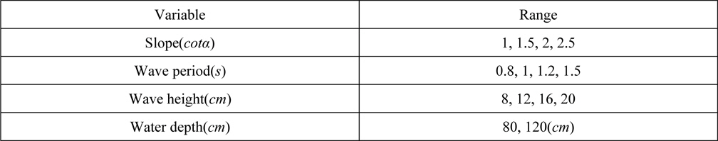
Definitions of main variables in laboratory tests.
In each numerical case, the wave maker signal height was firstly adjusted at the incident wave height. But, during a continuously sensing, the effect of reflected waves exactly in front of the RMB was analyzed. Comparing the recorded data in front of the RMB and the wanted wave characteristic in each test case, the appropriate correction was made in the input wave height of the wave maker. The values of run up were measured through the snapshot of the central section of breakwater, with a frequency of 0.2 seconds, and the value of the corresponding run up was measured. Particulary the run up measured is the distance between swl and the highest point of contact with the breakwater (Dentale et al., 2013).
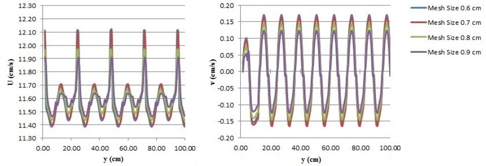
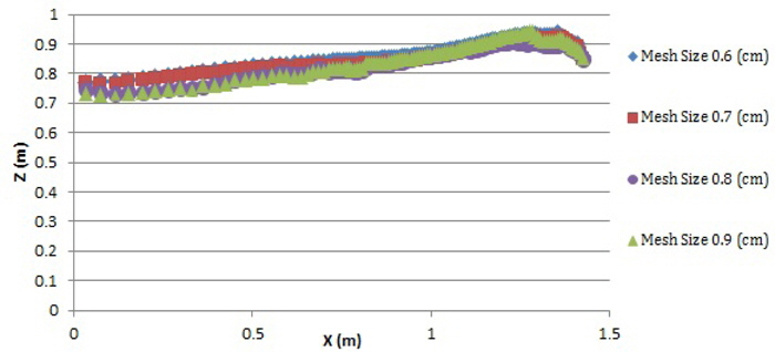
In order to obtain accurate results in the least amount of time, it is necessary to compute best mesh dimensions before simulation (Hsu et al., 2011). Grid independence is done to ensure that the solution is independent in terms of grid size. These grid independence tests were done applying 4 different sized meshes. Sizes of mesh tested in the experiment were as follows: 0.6
Results showed negligible difference in terms of mesh sizes 0.6 and 0.7
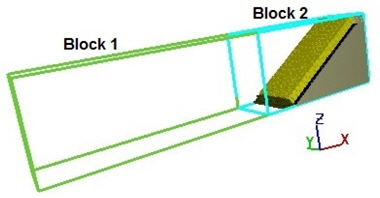
Due to the optimization of the design time, the zone was divided in two individual blocks, at wich differently precise grids have been used (see Fig. 6). The grid in the block1 was composed of 125000 cells, Δ
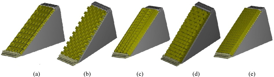
In order to study the effect of antifer placement pattern on wave run-up, the following mentioned 5 different placement patterns were studied: (regular, irregular A, irregular B, double pyramid and closed pyramid). In all 5 cases, antifer pieces were totally stable. Stability of the three first cases was investigated by Najafi-Jilani and Monshizadeh (2010) and the two remaining ones were studied by Frens (2007). These patterns are shown in Figs. 7-10.
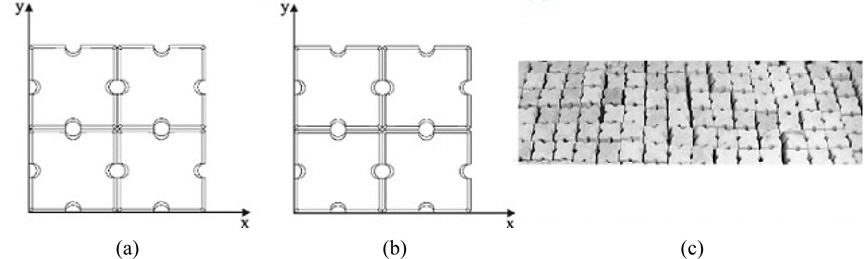
The regular pattern is equal to the ‘sloped wall placement pattern’ presented by (Yagci and Kapdasli, 2003). In the first layer, antifer-blocks were placed adjacent to each other with their grooves perpendicular to the slope. The second layer was placed straight onto the first layer using the same method. Figs. 7(a) and Figs.7(b) presents a top view of this method. In this figure the x-direction points along the slope and the y-direction points in an upward direction. (a) represents the first layer and (b) represents the second layer.
As shown in Fig. 8, irregular placement in A-Type is created by rotating the antifer units in the slope plane by about 45. The pattern, irregular placement B-Type, is made by rotating the antifer blocks around the normal axis of the slope.
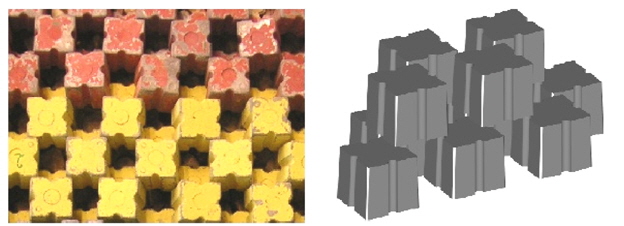
For the double pyramid method, the blocks of the first layer are placed by the regular pyramid pattern. The second layer was shifted horizontally compared to the first layer, so the blocks of the second layer are placed over the gaps of the first layer. The double pyramid pattern was indicated by Frens (2007). The double pyramid pattern is illustrated in Fig. 9.
Closed pyramid: The blocks in the first layer are placed with fixed horizontal distances from one another and in a regular position, with their grooves pendicular to the slope. The blocks of the second layer are placed diagonal for the first row directing to the left, for the second row to the right and so on. They fill up the gaps between the blocks of the first layer. The closed pyramid pattern is illustrated in Fig. 10.
Real porosity of the different placement patterns is presented in Table 2.
[Table 2] Real porosity of different placement pattern.

Real porosity of different placement pattern.
Fig. 11 shows breakwater sketches with 5 different placement patterns of antifer units.
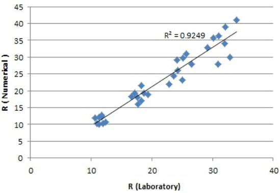
Experimental run-up results are compared with numerical simulation results in Fig. 12, and correlation coefficient R2 is computed. 92% correlation coefficient represents the fact that 3-dimensional direct simulation is able to simulate flow movement into porous medium well, and presents acceptable run-up.
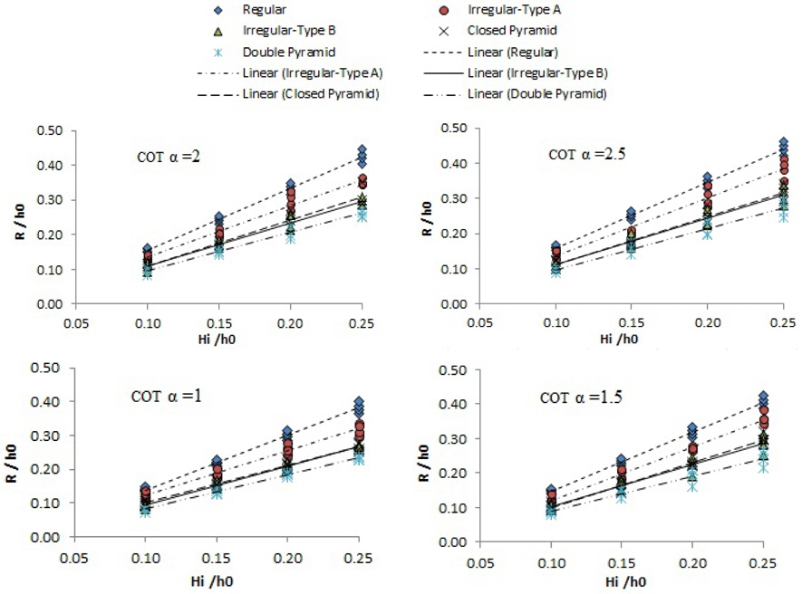
As previously mentioned, the main goal of investigations into wave run-up was to inspect the effect of placement pattern of antifer units on wave run-up. The variation of wave run-up vs. wave height for 5 different placement patterns of the antifer blocks is illustrated in Fig. 13.
The results show that effect of arrangement of antifer units on run-up value was significant, such that by changing the arrangement pattern from ordered to duplex pyramid, run-up was reduced by 35%. This reduction was observed for all 4 slopes (cotα = 1~ cotα = 2.5). However in steeper slopes, the effect of arrangement pattern on run-up reduction was more.
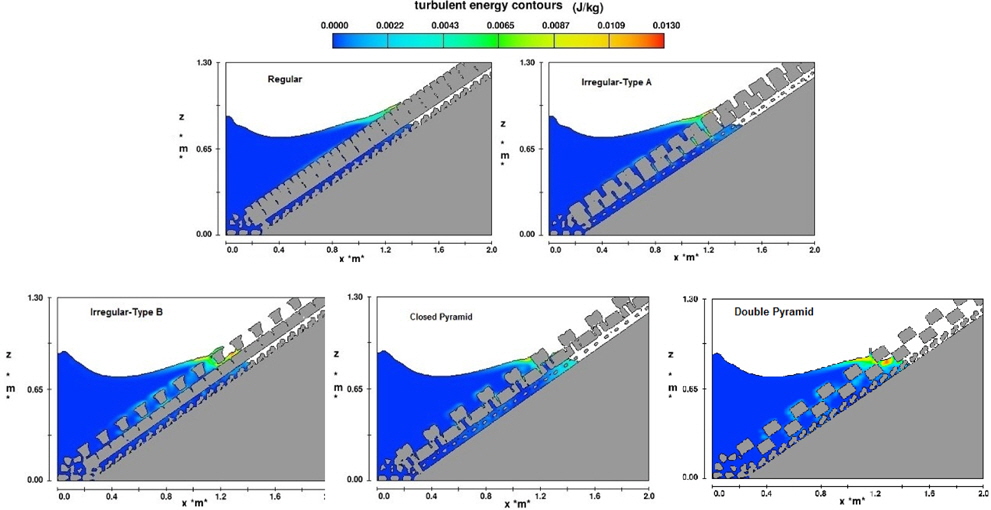
It is interesting that the closed pyramid arrangement, despite its higher porosity (more than 49% in the physical model) compared to the double pyramid arrangement, indicated more run-up values demonstrating the importance of the effect of coarseness and arrangement of armour pieces. In the figures below, turbulence energy near the armor layer is shown for a wave of 16
It is seen that turbulence energy among antifer blocks in a double pyramid arrangement is more than that of the closed pyramid arrangement, demonstrating that there is more energy amortization in this kind of arrangement and the importance of arrangement type over surface coarseness.
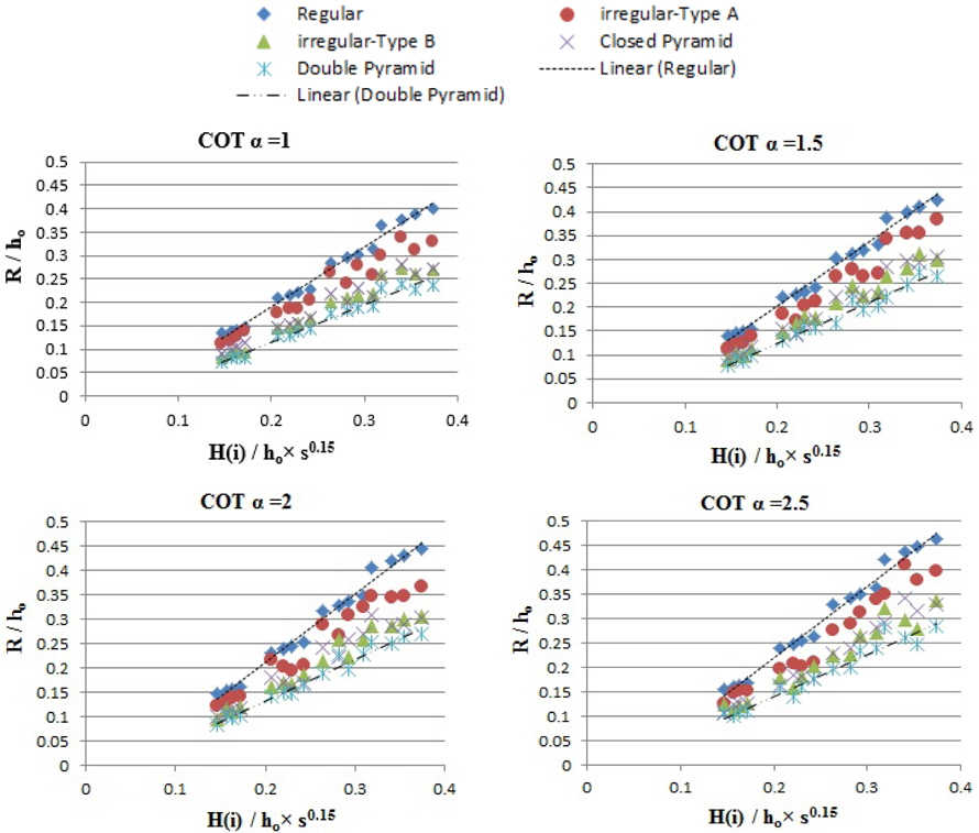
In order to study the effect of wave steepness,
In the present research, more than 320 numerical models were tested to investigate wave run-up on breakwaters covered by antifer armour units. Main variables were tested, they were as follows: antifer unit arrangement, breakwater slope, wave height and wave period. Results demonstrated better accuracy from using accurate geometry of a breakwater and application of the numerical method based on VOF algorithm e.g Flow3D, compared to numerical codes with coarseness coefficient and equivalent permeability.
The difference between the physical model and the numerical model is appreciable only when the relative wave height (incident wave height,